CreditMetrics: credit VaR from rating migrations

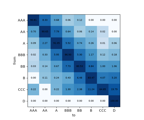
J. P. Morgan’s CreditMetrics (1997) revalues a bond in every rating it could hold a year from now, weights the values with a rating transition matrix, and reads the credit VaR off the resulting distribution. For a portfolio, obligors migrate jointly: each one’s asset return is mapped to a rating through normal thresholds, and the asset returns are correlated. The Technical Document’s five-year BBB bond has mean value 107.09 and standard deviation 2.99.

import matplotlib.pyplot as plt
import numpy as np

from financialkit.credit import (
    RATINGS,
    creditmetrics_bbb_values,
    creditmetrics_bond,
    creditmetrics_matrix,
    creditmetrics_portfolio,
    joint_migration_probabilities,
    migration_thresholds,
)
from financialkit.credit.visualizers import plot_transition_matrix, plot_value_distribution

P = creditmetrics_matrix()
plot_transition_matrix(P, labels=RATINGS)

<Axes: xlabel='to', ylabel='from'>

One BBB bond

bond = creditmetrics_bond(creditmetrics_matrix(normalize=False)[3], creditmetrics_bbb_values())
print(f"mean {bond.mean:.2f}, std {bond.std:.2f}, 1% percentile {bond.percentile(0.01):.2f}, 99% credit VaR {bond.credit_var(0.99):.2f}")
plot_value_distribution(bond, labels=RATINGS)
print("BBB thresholds (z):", np.round(migration_thresholds(P[3])[1:-1], 2))

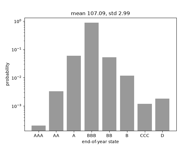
mean 107.09, std 2.99, 1% percentile 98.10, 99% credit VaR 8.99
BBB thresholds (z): [ 3.54  2.7   1.53 -1.49 -2.18 -2.75 -2.91]

Two obligors: joint migrations

for rho in (0.0, 0.3, 0.6):
    J = joint_migration_probabilities(P[3], P[2], rho)
    print(f"rho = {rho:.1f}: P(both default) = {J[-1, -1]:.2e}, P(both unchanged) = {J[3, 2]:.4f}")

rho = 0.0: P(both default) = 1.08e-06, P(both unchanged) = 0.7915
rho = 0.3: P(both default) = 1.56e-05, P(both unchanged) = 0.7969
rho = 0.6: P(both default) = 9.63e-05, P(both unchanged) = 0.8131

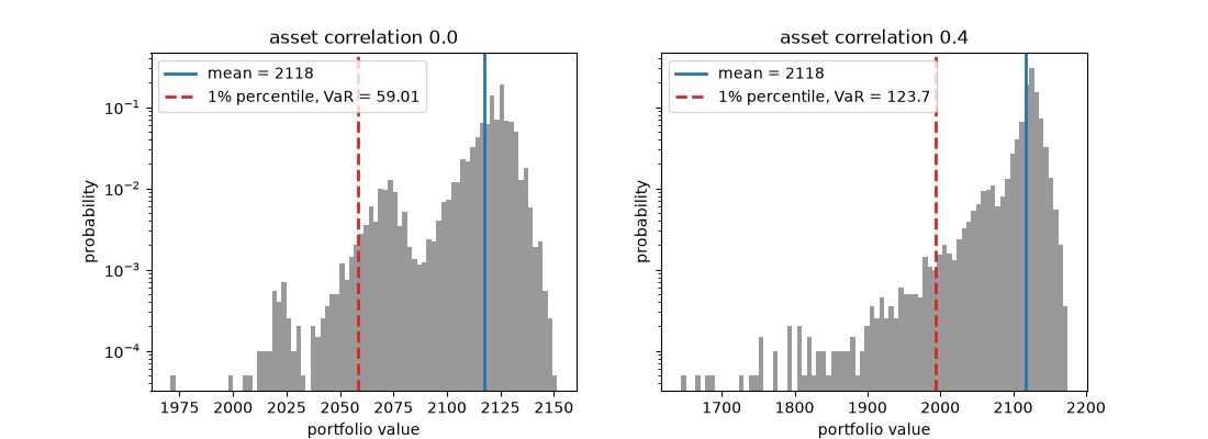
A 20-bond portfolio

Correlation fattens the left tail of the portfolio value.

ratings = np.repeat([2, 3, 4], [7, 7, 6])
fig, ax = plt.subplots(1, 2, figsize=(11, 4), sharey=True)
for a, rho in zip(ax, (0.0, 0.4), strict=True):
    res = creditmetrics_portfolio(P, ratings, creditmetrics_bbb_values(), rho, 20000, rng=0)
    plot_value_distribution(res, ax=a, bins=80)
    a.set_title(f"asset correlation {rho}")
    a.set_yscale("log")

plt.show()