Altman’s Z-score

Altman (1968) fed five accounting ratios of 33 bankrupt and 33 surviving manufacturers into a linear discriminant analysis and found

\[Z = 1.2 X_1 + 1.4 X_2 + 3.3 X_3 + 0.6 X_4 + 1.0 X_5,\]

with working capital, retained earnings, EBIT and sales scaled by total assets and market equity scaled by total liabilities. Below 1.81 a firm is in the distress zone, above 2.99 it is safe. Here a synthetic sample of healthy and failing firms is scored, and Fisher’s discriminant re-estimated from the same ratios gives weights in the same direction.

import matplotlib.pyplot as plt
import numpy as np

from financialkit.credit import ALTMAN_COEFFICIENTS, altman_ratios, altman_z_score, altman_zone, linear_discriminant

rng = np.random.default_rng(0)


def firms(n, healthy):
    """Synthetic balance sheets: failing firms have thin working capital, losses and high leverage."""
    ta = rng.lognormal(6, 0.5, n)
    shift = 1.0 if healthy else -1.0
    wc = ta * (0.15 + 0.12 * shift + 0.10 * rng.standard_normal(n))
    re = ta * (0.15 + 0.25 * shift + 0.15 * rng.standard_normal(n))
    ebit = ta * (0.03 + 0.08 * shift + 0.05 * rng.standard_normal(n))
    tl = ta * np.clip(0.55 - 0.2 * shift + 0.1 * rng.standard_normal(n), 0.1, None)
    me = tl * np.exp(0.2 + 0.8 * shift + 0.4 * rng.standard_normal(n))
    sales = ta * np.clip(1.4 + 0.3 * shift + 0.3 * rng.standard_normal(n), 0.1, None)
    return wc, re, ebit, me, sales, ta, tl


good, bad = firms(400, True), firms(400, False)
z_good, z_bad = altman_z_score(*good), altman_z_score(*bad)

Z-scores and Altman’s zones

fig, ax = plt.subplots(figsize=(8, 4))
bins = np.linspace(-4, 10, 70)
ax.hist(z_good, bins, alpha=0.6, label="survivors")
ax.hist(z_bad, bins, alpha=0.6, label="failed")
ax.axvspan(bins[0], 1.81, color="C3", alpha=0.08)
ax.axvspan(2.99, bins[-1], color="C2", alpha=0.08)
ax.axvline(1.81, color="C3", ls="--")
ax.axvline(2.99, color="C2", ls="--")
ax.set_xlabel("Z-score")
ax.set_ylabel("firms")
ax.set_title("distress zone < 1.81 < grey zone < 2.99 < safe zone")
ax.legend()

for name, z in (("survivors", z_good), ("failed", z_bad)):
    zones = altman_zone(z)
    print(f"{name:9s}: " + ", ".join(f"{k} {np.mean(zones == k):.0%}" for k in ("distress", "grey", "safe")))

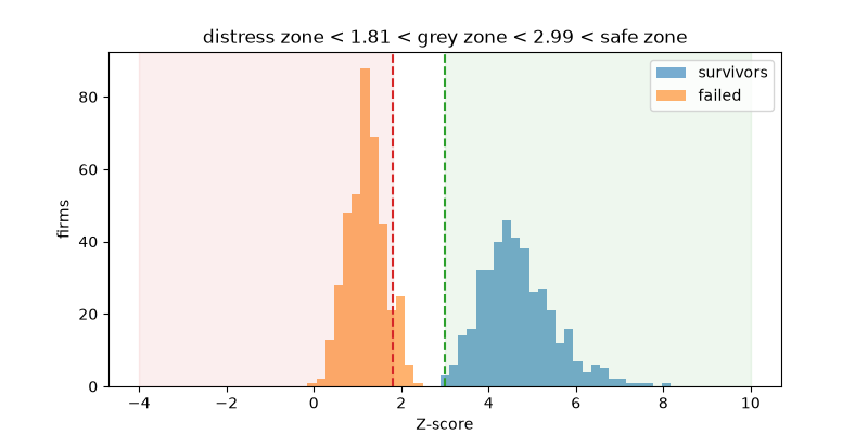
survivors: distress 0%, grey 0%, safe 100%
failed   : distress 89%, grey 11%, safe 0%

Re-estimating the discriminant

Fisher’s linear discriminant is defined only up to scale, so compare directions: normalise both weight vectors.

w, cutoff = linear_discriminant(altman_ratios(*good), altman_ratios(*bad))
print("Altman weights (normalised):", np.round(ALTMAN_COEFFICIENTS / np.linalg.norm(ALTMAN_COEFFICIENTS), 2))
print("Fisher weights (normalised):", np.round(w / np.linalg.norm(w), 2))

plt.show()

Altman weights (normalised): [0.3  0.35 0.83 0.15 0.25]
Fisher weights (normalised): [0.33 0.36 0.87 0.04 0.11]