Longstaff-Schwartz least-squares Monte Carlo

Monte Carlo simulates forward, but early exercise is decided backward: whether to exercise today depends on the value of waiting. Francis Longstaff and Eduardo Schwartz (2001) estimated that continuation value by regressing the discounted future cash flows of the in-the-money paths on a few functions of today’s price. Working back from expiry, each path is exercised where the payoff beats the fitted value. The method extends to many assets and path-dependent payoffs, where trees and PDEs give up.

import matplotlib.pyplot as plt
import numpy as np

from financialkit.exotic_options import longstaff_schwartz, plot_exercise_boundary, regression_basis
from financialkit.integrators import gbm_paths
from financialkit.options import CRRTree, black_scholes_price

S, K, T, r, sigma = 36.0, 40.0, 1.0, 0.06, 0.2

One regression step

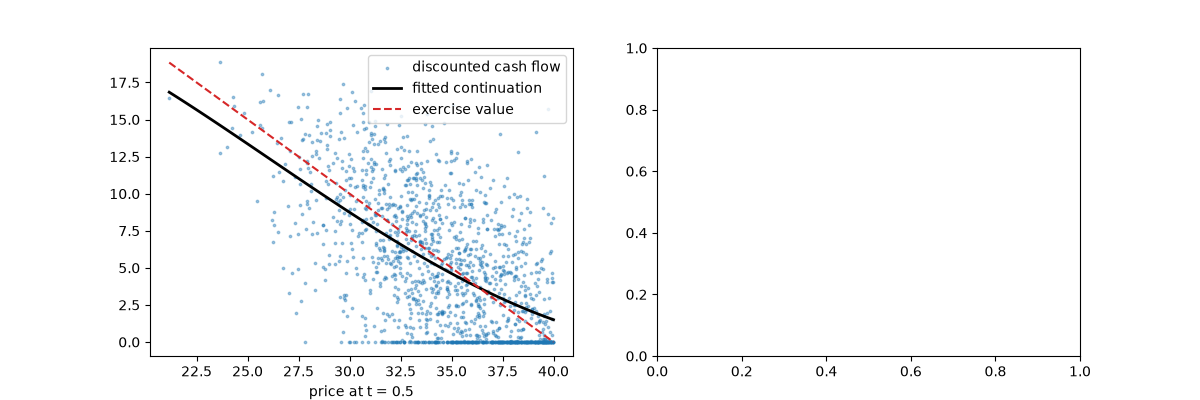
At t = 0.5 the discounted value of exercising optimally later (approximated here by the European put to expiry) is scattered against the price, with the fitted continuation value.

_, paths = gbm_paths(S, r, sigma, T, 2, 2000, rng=0)
St = paths[:, 1]
y = np.exp(-r * 0.5) * np.maximum(K - paths[:, 2], 0.0)
itm = St < K
coef, *_ = np.linalg.lstsq(regression_basis(St[itm] / K), y[itm], rcond=None)
grid = np.linspace(St[itm].min(), K, 100)
fig, axes = plt.subplots(1, 2, figsize=(12, 4))
axes[0].scatter(St[itm], y[itm], s=3, alpha=0.4, label="discounted cash flow")
axes[0].plot(grid, regression_basis(grid / K) @ coef, "k", lw=2, label="fitted continuation")
axes[0].plot(grid, K - grid, "C3--", label="exercise value")
axes[0].set_xlabel("price at t = 0.5")
axes[0].legend()

<matplotlib.legend.Legend object at 0x116d92e40>

Price and exercise boundary against the binomial tree

Longstaff and Schwartz’s Table 1: the finite-difference value with 50 exercise dates is 4.478.

res = longstaff_schwartz(S, K, T, r, sigma, n_exercise=50, n_paths=20_000, rng=1)
tree = CRRTree(500).price(S, K, T, r, sigma, option_type="put", american=True)
european = black_scholes_price(S, K, T, r, sigma, option_type="put")
print(f"Longstaff-Schwartz {res.estimate:.4f} +/- {res.std_error:.4f}; tree {tree.price:.4f}; European {european:.4f}")
print(f"paths exercised early: {res.exercise_probability:.1%}")
plot_exercise_boundary(res, ax=axes[1])
axes[1].plot(tree.times, tree.exercise_boundary, "k", lw=1, label="CRR tree")
axes[1].set_ylim(30, 41)
axes[1].legend()
fig.tight_layout()
plt.show()

Longstaff-Schwartz 4.4687 +/- 0.0134; tree 4.4864; European 3.8443
paths exercised early: 69.7%