Stulz options on the maximum and minimum

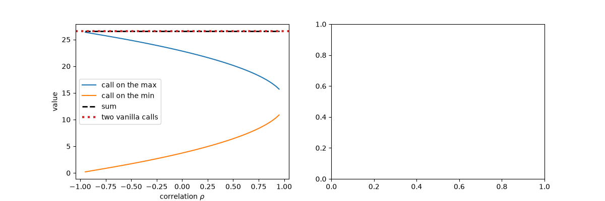
Rene Stulz (1982) priced calls and puts on the better or the worse of two assets, \((\max(S_1, S_2) - K)^+\) and \((\min(S_1, S_2) - K)^+\), the simplest “rainbow” options. The answer needs the bivariate normal distribution. Because \(\max + \min = S_1 + S_2\), the two calls always add up to the two vanilla calls, and correlation moves value between them: diversification makes the maximum more valuable and the minimum less.

import matplotlib.pyplot as plt
import numpy as np

from financialkit.exotic_options import stulz_price
from financialkit.options import black_scholes_price

S1, S2, K, T, r, s1, s2 = 100.0, 100.0, 100.0, 1.0, 0.05, 0.25, 0.3
rho = np.linspace(-0.95, 0.95, 60)

fig, axes = plt.subplots(1, 2, figsize=(12, 4))
cmax = stulz_price(S1, S2, K, T, r, s1, s2, rho, kind="max")
cmin = stulz_price(S1, S2, K, T, r, s1, s2, rho, kind="min")
vanilla = black_scholes_price(S1, K, T, r, s1) + black_scholes_price(S2, K, T, r, s2)
axes[0].plot(rho, cmax, label="call on the max")
axes[0].plot(rho, cmin, label="call on the min")
axes[0].plot(rho, cmax + cmin, "k--", lw=2, label="sum")
axes[0].axhline(vanilla, color="C3", ls=":", lw=3, label="two vanilla calls")
axes[0].set_xlabel(r"correlation $\rho$")
axes[0].set_ylabel("value")
axes[0].legend()

<matplotlib.legend.Legend object at 0x11713d160>

Puts on the maximum and minimum across strikes

Ks = np.linspace(70.0, 130.0, 60)
for kind in ("max", "min"):
    axes[1].plot(Ks, stulz_price(S1, S2, Ks, T, r, s1, s2, 0.5, option_type="put", kind=kind), label=f"put on the {kind}")
axes[1].plot(Ks, black_scholes_price(S1, Ks, T, r, s1, option_type="put"), "k:", label="put on asset 1")
axes[1].set_xlabel("strike K")
axes[1].legend()
fig.tight_layout()
plt.show()