Amihud’s illiquidity ratio

Yakov Amihud (2002) proposed a liquidity measure that needs only daily returns and dollar volume: the average of \(|r_d| / \mathrm{DVol}_d\), the price move per dollar traded. It approximates Kyle’s lambda, which needs signed order flow, and Amihud found that stocks with a higher ratio earn higher expected returns, an illiquidity premium.

import matplotlib.pyplot as plt
import numpy as np
from scipy import stats

from financialkit.market_microstructure import amihud_illiquidity, kyle_lambda

rng = np.random.default_rng(15)

A cross-section of stocks

Each stock’s daily return is its Kyle lambda times its signed dollar order flow plus public news. Lambdas span two orders of magnitude, and less liquid stocks trade less.

n_stocks, days = 80, 250
lam = 10 ** rng.uniform(-9, -7, n_stocks)  # return per dollar of net order flow
scale = 2e5 / np.sqrt(lam / 1e-9)  # typical net flow in dollars
amihud, kyle = [], []
for i in range(n_stocks):
    net = scale[i] * rng.standard_normal(days)
    dvol = np.abs(net) + scale[i] * rng.gamma(2.0, 1.0, days)
    r = lam[i] * net + 0.005 * rng.standard_normal(days)
    amihud.append(amihud_illiquidity(r, dvol))
    kyle.append(kyle_lambda(r, net).coef[1])

rho = stats.spearmanr(lam, amihud).statistic
print(f"rank correlation between Amihud's ratio and the true lambda: {rho:.2f}")

fig, ax = plt.subplots(figsize=(6, 4.5))
ax.loglog(lam, amihud, "o", color="C0", label="Amihud ratio (per $1M)")
ax.loglog(lam, 1e6 * np.abs(kyle), "x", color="C1", label="regression lambda (per $1M)")
ax.set_xlabel("true Kyle lambda")
ax.set_ylabel("estimate")
ax.legend()
fig.tight_layout()

plt.show()

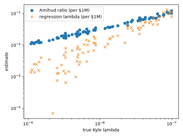
rank correlation between Amihud's ratio and the true lambda: 0.99