Grinold’s fundamental law of active management

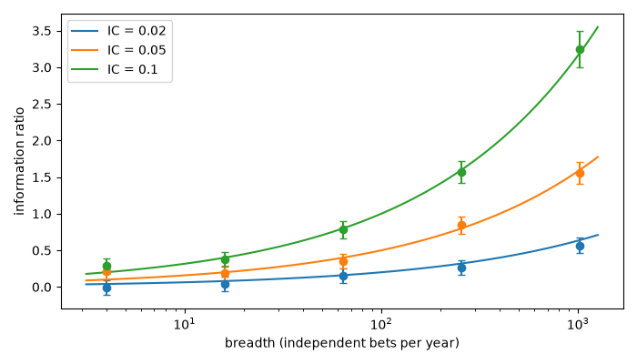
Richard Grinold (1989) decomposed an active manager’s information ratio into skill and breadth:

\[IR \approx IC \sqrt{BR},\]

where the information coefficient \(IC\) is the correlation between forecasts and outcomes and the breadth \(BR\) is the number of independent forecasts a year. A tiny edge applied to many independent bets beats a large edge applied to a few: an IC of 0.05 on 400 stocks gives the same IR as an IC of 0.5 on four markets.

import matplotlib.pyplot as plt
import numpy as np

from financialkit.portfolio import fundamental_law, simulate_active_management

Simulated managers against the law

Each manager makes breadth independent bets a year for 400 years. The exact IR of this model, \(IC\sqrt{BR}/\sqrt{1 + IC^2}\), is barely below Grinold’s first-order law.

breadths = np.array([4, 16, 64, 256, 1024])
fig, ax = plt.subplots(figsize=(7, 4))
for k, ic in enumerate([0.02, 0.05, 0.1]):
    sims = [simulate_active_management(ic, int(b), 400, rng=k * 10 + i) for i, b in enumerate(breadths)]
    ax.errorbar(breadths, [s.ir for s in sims], yerr=[2 * s.ir_se for s in sims], fmt="o", color=f"C{k}", capsize=3)
    bb = np.logspace(0.5, 3.1, 100)
    ax.plot(bb, fundamental_law(ic, bb), color=f"C{k}", label=f"IC = {ic}")
ax.set_xscale("log")
ax.set_xlabel("breadth (independent bets per year)")
ax.set_ylabel("information ratio")
ax.legend()
fig.tight_layout()

Same IR, different businesses

for ic, br in [(0.5, 4), (0.1, 100), (0.05, 400), (0.02, 2500)]:
    res = simulate_active_management(ic, br, 2000, rng=1)
    print(f"IC {ic:<4} x sqrt({br:>4}) = {fundamental_law(ic, br):.2f}; simulated IR {res.ir:.2f} +/- {res.ir_se:.2f}")
plt.show()

IC 0.5  x sqrt(   4) = 1.00; simulated IR 0.90 +/- 0.03
IC 0.1  x sqrt( 100) = 1.00; simulated IR 0.98 +/- 0.03
IC 0.05 x sqrt( 400) = 1.00; simulated IR 0.96 +/- 0.03
IC 0.02 x sqrt(2500) = 1.00; simulated IR 1.00 +/- 0.03