physicskit: Computational Physics in Python

physicskit is a unified scientific toolkit for computational physics, spanning 14 domains – from stellar dynamics to quantum entanglement – under one NumPy-based API. It’s built for physics students working through a textbook problem, curious learners exploring a topic on their own, and educators building a demonstration: every subpackage is called, tested, and visualized the same way, so moving from classical mechanics to condensed matter to general relativity means picking up new physics, not a new set of conventions. Units stay native to the field instead: \(G=1\) for orbits, \(\hbar=1\) for quantum states, \(k_B=1\) for statistical mechanics, matching how the papers you’re checking against actually write it, rather than forcing everything through SI. Units and conventions lists each subpackage’s convention and shows how physicskit.units converts results to SI once you choose the physical scale.

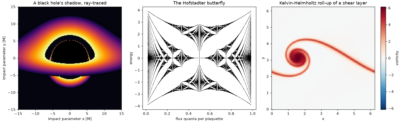
Every subpackage is grounded in the physics it implements, not just coded against it: public functions carry runnable, CI-checked examples, and each subpackage’s history page traces the breakthroughs behind it – from Huygens’ 1690 wave construction to the 2017 GW170817 neutron-star chirp – each one linked to the code that reproduces it. The goal is a toolkit you can trust to move between domains without re-deriving the plumbing every time:

• physicskit.astro – stellar structure, N-body dynamics, orbital mechanics, galactic dynamics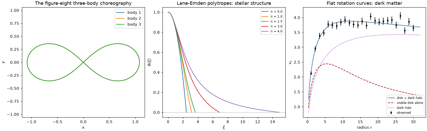

  

• physicskit.chaos – chaotic dynamical systems and 2D quantum billiards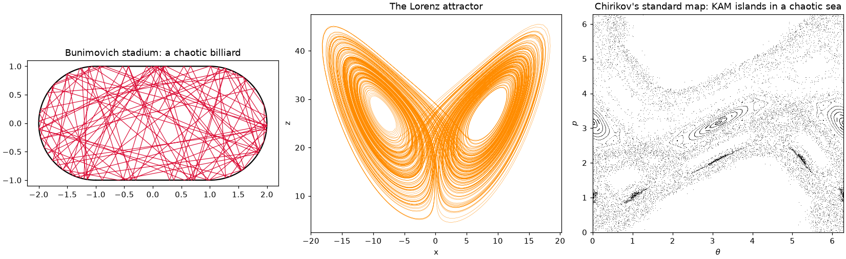

  

• physicskit.classical – classical (Newtonian/Lagrangian/Hamiltonian) mechanics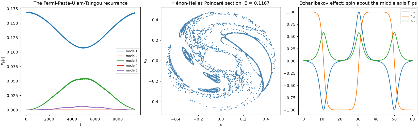

  

• physicskit.condensed – tight-binding models, topological band theory, superconductivity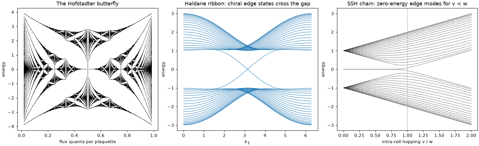

  

• physicskit.fields – electrodynamics (FDTD), solitons, BEC vortex lattices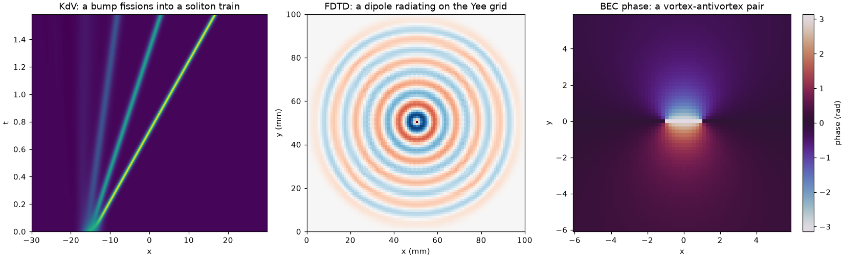

  

• physicskit.fluids – potential flow, viscous flow, vortex dynamics, instabilities, compressible flow, Navier-Stokes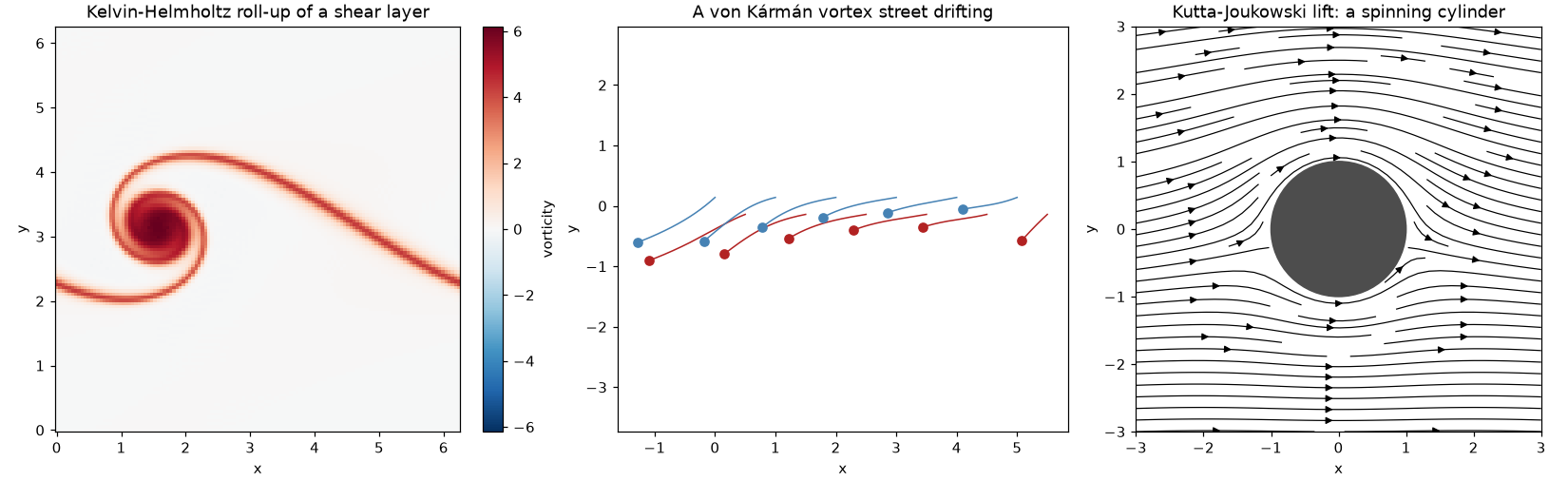

  

• physicskit.optics – ray/wave/Gaussian-beam optics, Wigner functions, Jaynes-Cummings dynamics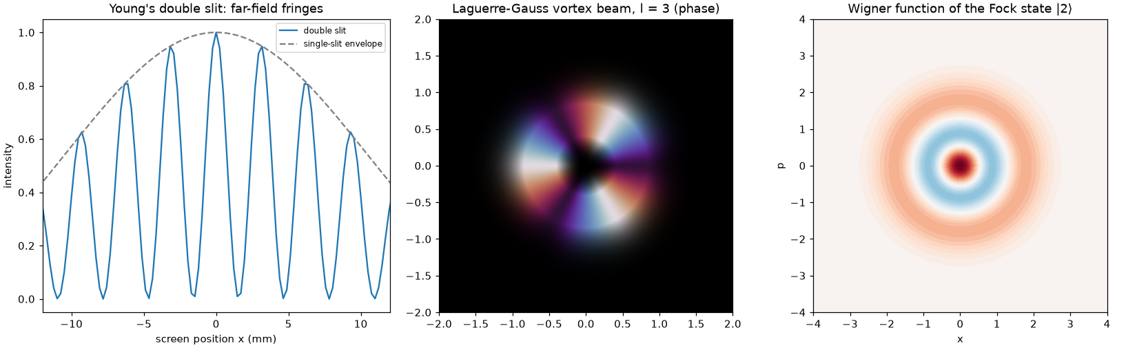

  

• physicskit.particle – relativistic kinematics, two-body decays, scattering, nuclear physics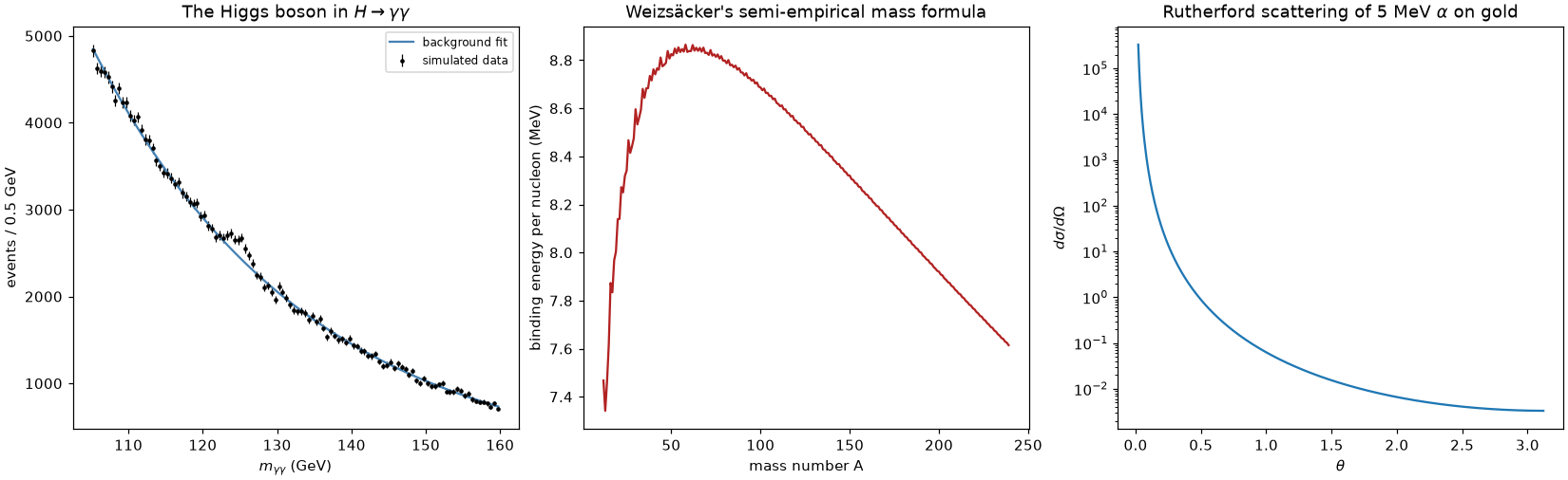

  

• physicskit.plasma – single-particle motion, magnetohydrodynamics, cold-plasma waves, kinetic theory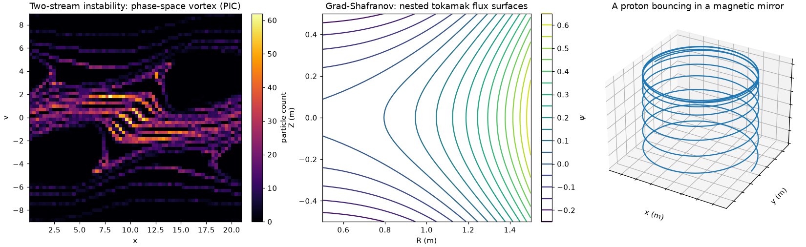

  

• physicskit.quantum – quantum mechanics: wave packets, potentials, entanglement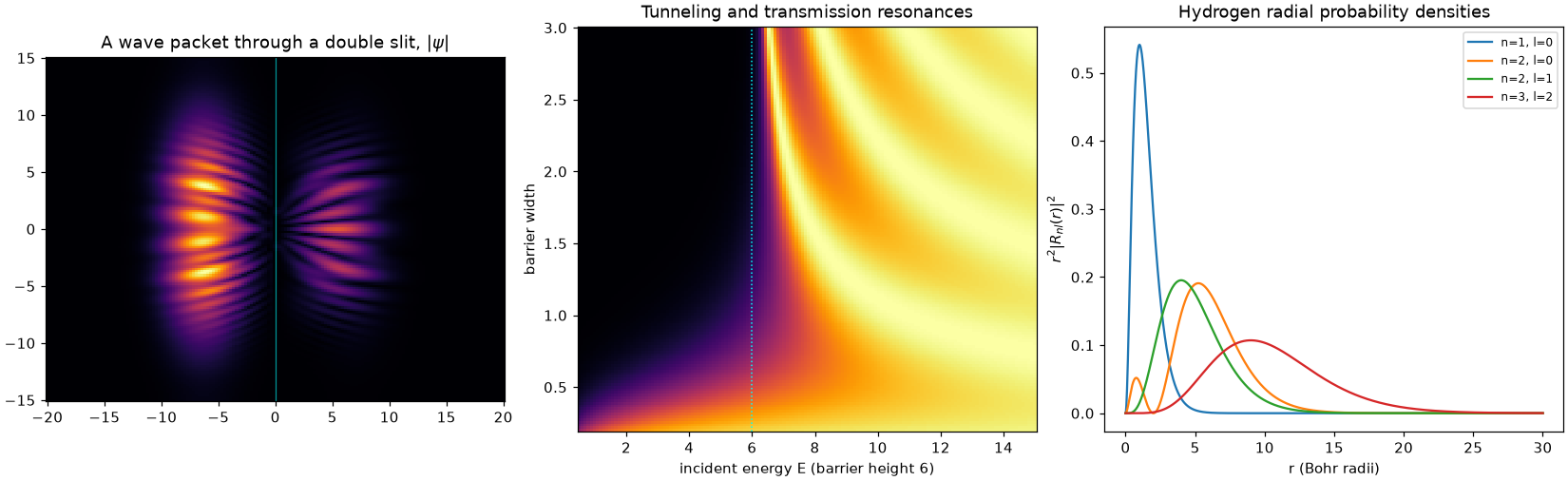

  

• physicskit.relativity – numerical general relativity: black holes, lensing, gravitational waves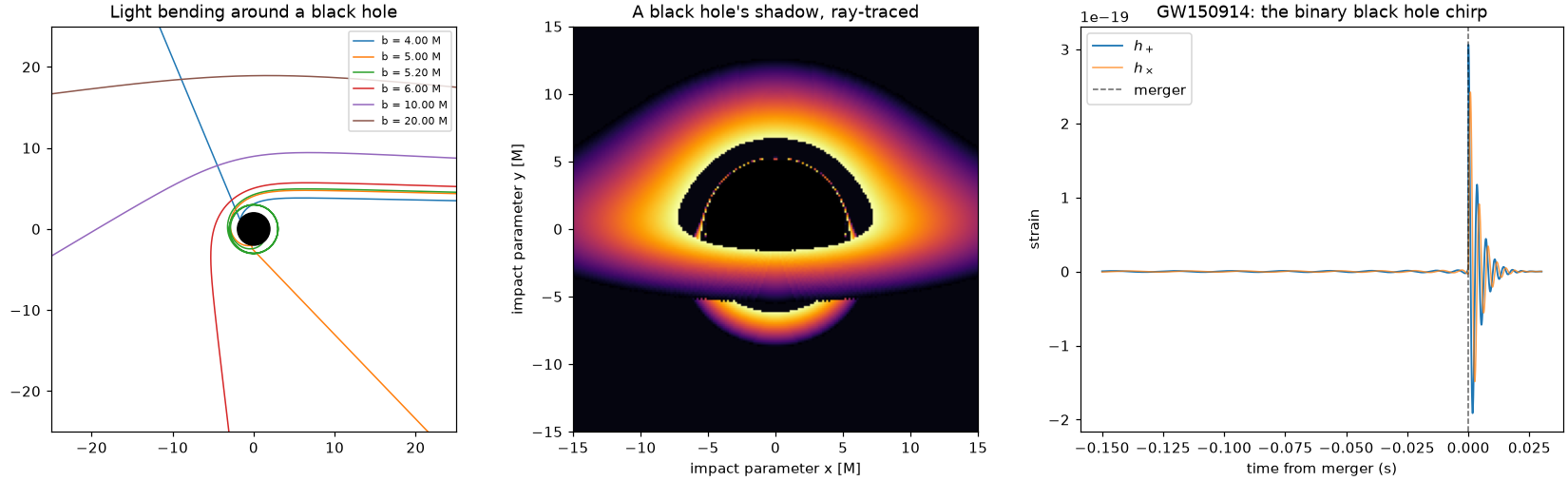

  

• physicskit.rmt – random matrix theory, organized around Dyson’s threefold way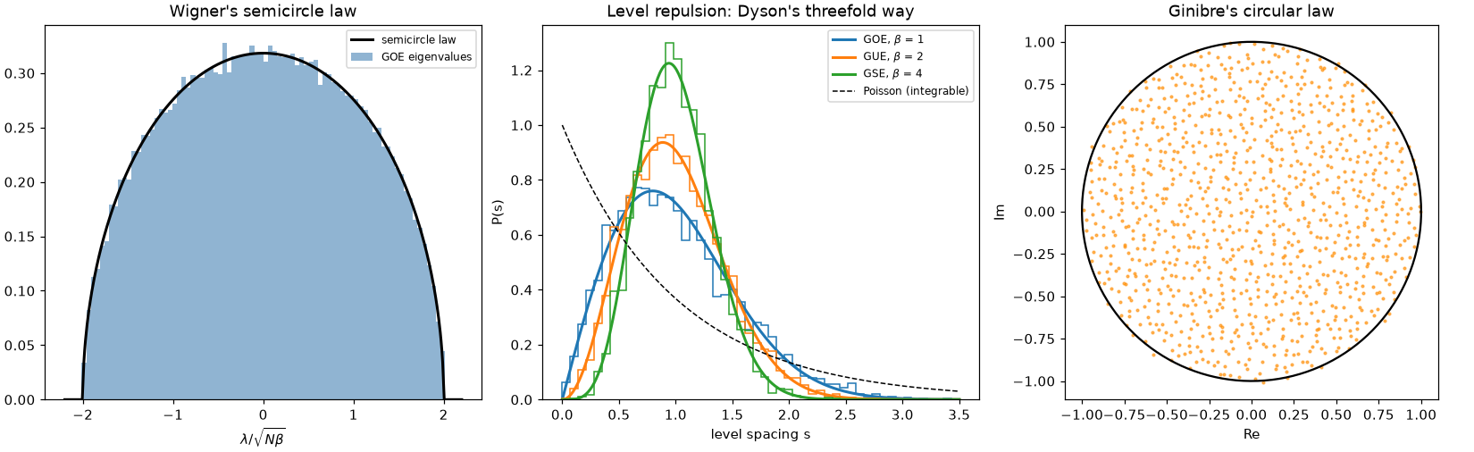

  

• physicskit.semiclassical – WKB/EBK quantization, semiclassical propagators, the Gutzwiller trace formula, and quantum scarring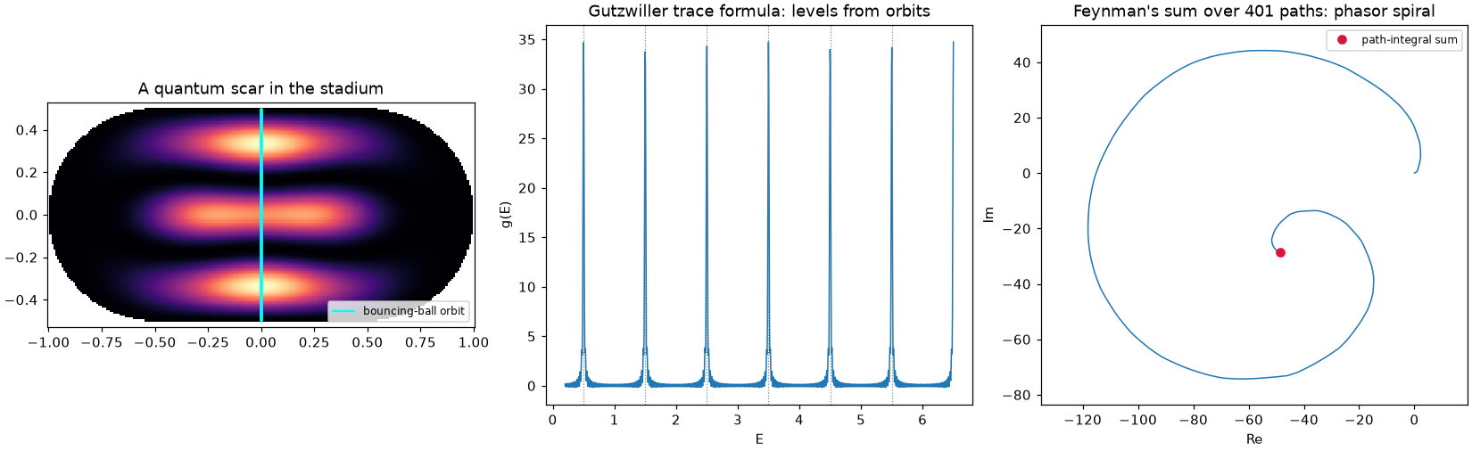

  

• physicskit.statphys – statistical mechanics: lattice models, molecular dynamics, criticality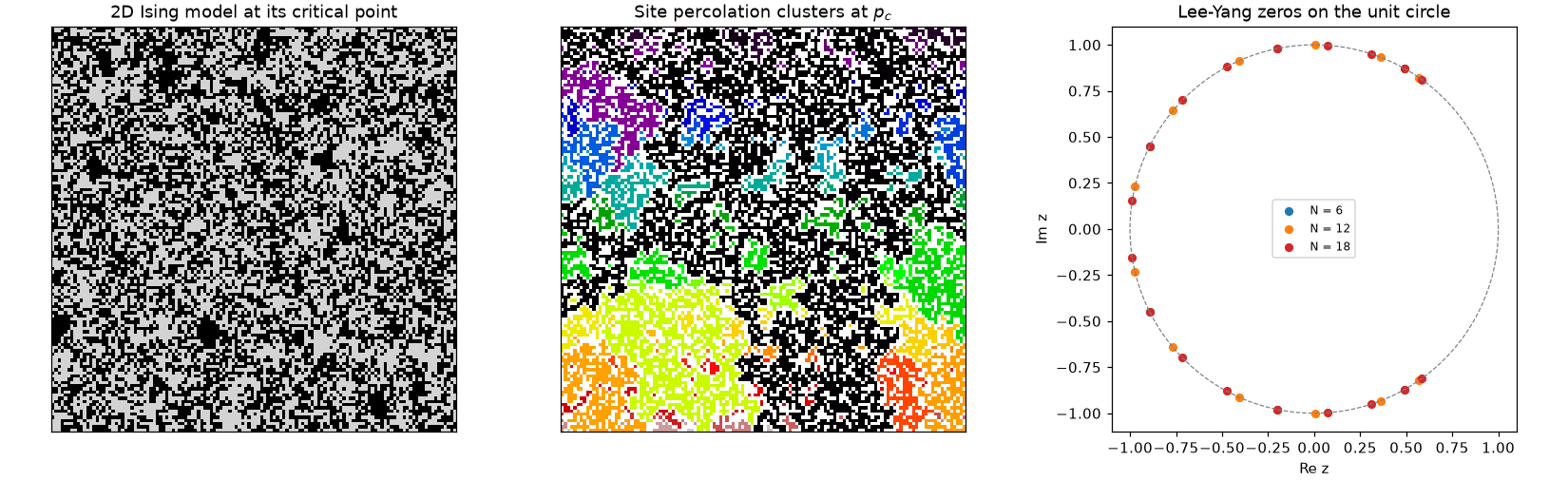

  

Important

Each domain is a teaching-depth subset of its field, not a complete implementation. physicskit is not a replacement for specialist libraries in production work: for that, use the dedicated tools (SciPy, QuTiP, Astropy, REBOUND, Kwant, PlasmaPy, and the like) directly.

physicskit is part of a family of packages – physicskit, mathematicskit and chemistrykit – that share the same architecture, API conventions, and history-driven documentation. For tight-binding models beyond physicskit.condensed – arbitrary finite lattices, ribbons and defects, non-Hermitian bands, Landauer transport, and the kernel polynomial method for very large samples – see the dedicated package tbkit.

Conventionally imported as pk:

import physicskit as pk
import numpy as np

H = lambda k1, k2: pk.condensed.haldane_model(k1, k2, phi=np.pi / 2)
chern_numbers = pk.condensed.compute_chern_number(H, grid_size=30)
print(chern_numbers)  # [1, -1]

Related toolkits

Sibling Python toolkits for learning and teaching, built the same way:

• blockchainkit – cryptography, consensus and blockchain systems

• chemistrykit – computational chemistry

• engineeringkit – computational engineering

• financialkit – quantitative finance

• mathematicskit – computational mathematics

• tbkit – tight-binding models, band topology and quantum transport