Harrison-Kreps: state prices and the stochastic discount factor

Michael Harrison and David Kreps (1979) proved the fundamental theorem of asset pricing: a market has no arbitrage if and only if some strictly positive linear rule prices every traded payoff. With finitely many states it is a vector of state prices \(q_s > 0\) with \(p = X'q\); divided by the physical probabilities it is the stochastic discount factor \(m_s = q_s / \pi_s\), so that \(p = E[m x]\); normalised, it is the risk-neutral measure. In a complete market the state prices are unique. In an incomplete one, a new claim has an interval of arbitrage-free prices.

import matplotlib.pyplot as plt
import numpy as np

from financialkit.asset_pricing import FiniteStateMarket

# A one-period binomial market: bond and stock.
S0, R = 100.0, 1.03
up_down = np.array([125.0, 85.0])
mkt = FiniteStateMarket(np.column_stack([[R, R], up_down]), [1.0, S0], probabilities=[0.6, 0.4])
print("complete:", mkt.is_complete, " arbitrage free:", mkt.is_arbitrage_free())
print("state prices:", mkt.state_prices().round(4), " risk-neutral:", mkt.risk_neutral_probabilities().round(4))
print("SDF:", mkt.sdf().round(4))

complete: True  arbitrage free: True
state prices: [0.4369 0.534 ]  risk-neutral: [0.45 0.55]
SDF: [0.7282 1.335 ]

An arbitrage when the stock is mispriced

bad = FiniteStateMarket(np.column_stack([[R, R], up_down]), [1.0, 80.0])
theta = bad.arbitrage_portfolio()
theta = theta / theta[1]  # per share bought
print(f"stock at 80: arbitrage free? {bad.is_arbitrage_free()}")
print(f"buy 1 share, hold {theta[0]:+.1f} bonds: cost {bad.prices @ theta:+.2f}, payoffs {(bad.payoffs @ theta).round(2)}")

stock at 80: arbitrage free? False
buy 1 share, hold -80.0 bonds: cost +0.00, payoffs [42.6  2.6]

Incompleteness: a trinomial market

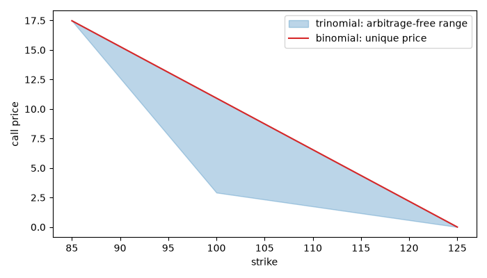
Three states and two assets: the state prices are no longer unique, and each call has a range of prices consistent with no arbitrage. The binomial price lies inside it.

states = np.array([125.0, 100.0, 85.0])
tri = FiniteStateMarket(np.column_stack([np.full(3, R), states]), [1.0, S0])
strikes = np.linspace(85, 125, 41)
bounds = np.array([tri.price_bounds(np.maximum(states - K, 0)) for K in strikes])
binom = np.array([mkt.state_prices() @ np.maximum(up_down - K, 0) for K in strikes])

fig, ax = plt.subplots(figsize=(7, 4))
ax.fill_between(strikes, bounds[:, 0], bounds[:, 1], color="C0", alpha=0.3, label="trinomial: arbitrage-free range")
ax.plot(strikes, binom, "C3", label="binomial: unique price")
ax.set_xlabel("strike")
ax.set_ylabel("call price")
ax.legend()
fig.tight_layout()

plt.show()