The Hansen-Jagannathan bound

Lars Peter Hansen and Ravi Jagannathan (1991) asked what asset returns alone reveal about the stochastic discount factor. Any \(m\) that prices the returns, \(E[m R] = 1\), must satisfy

\[\frac{\sigma(m)}{E(m)} \ge \frac{|E[R^e]|}{\sigma(R^e)}\]

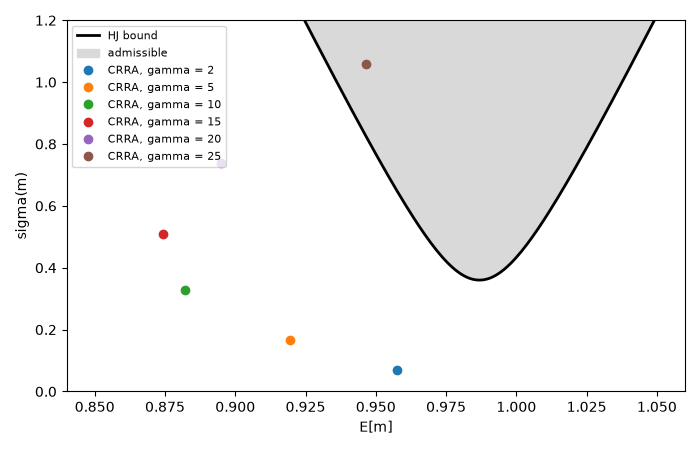
for every excess return \(R^e\). With US stocks’ Sharpe ratio of about 0.4 a year, the discount factor must vary by about 40% a year. The power-utility SDF \(\beta (C_{t+1}/C_t)^{-\gamma}\) varies by about \(\gamma \sigma_c\), roughly \(0.036\gamma\), so it enters the admissible region only for \(\gamma\) around 25, and on the way it passes through riskless rates \(1/E(m) - 1\) above 10%.

stock Sharpe ratio over bills: 0.36
 CRRA, gamma = 2: E[m] = 0.957, sigma(m) = 0.069, admissible: False
 CRRA, gamma = 5: E[m] = 0.920, sigma(m) = 0.167, admissible: False
CRRA, gamma = 10: E[m] = 0.882, sigma(m) = 0.328, admissible: False
CRRA, gamma = 15: E[m] = 0.874, sigma(m) = 0.509, admissible: False
CRRA, gamma = 20: E[m] = 0.895, sigma(m) = 0.738, admissible: False
CRRA, gamma = 25: E[m] = 0.946, sigma(m) = 1.057, admissible: True

import matplotlib.pyplot as plt
import numpy as np

from financialkit.asset_pricing import LucasTree, hansen_jagannathan_bound, max_sharpe_ratio
from financialkit.asset_pricing.visualizers import plot_hj_bound

# Annual gross returns of stocks and bills, Mehra-Prescott sample moments.
mu = np.array([1.0698, 1.0080])
vol = np.array([0.1654, 0.0567])
cov = np.array([[1.0, 0.1], [0.1, 1.0]]) * np.outer(vol, vol)
bound = hansen_jagannathan_bound(mu, cov, np.linspace(0.85, 1.05, 200))
print(f"stock Sharpe ratio over bills: {max_sharpe_ratio([mu[0] - mu[1]], [[cov[0, 0] - 2 * cov[0, 1] + cov[1, 1]]]):.2f}")

models = {}
for g in (2, 5, 10, 15, 20, 25):
    models[f"CRRA, gamma = {g}"] = LucasTree(0.99, g, 0.018, 0.036).moments()

fig, ax = plt.subplots(figsize=(7, 4.5))
plot_hj_bound(bound, models, ax=ax)
for name, m in models.items():
    print(f"{name:>16}: E[m] = {m.sdf_mean:.3f}, sigma(m) = {m.sdf_vol:.3f}, admissible: {bound.admits(m.sdf_mean, m.sdf_vol)}")
ax.set_ylim(0, 1.2)
fig.tight_layout()

plt.show()