Kemna-Vorst Asian options

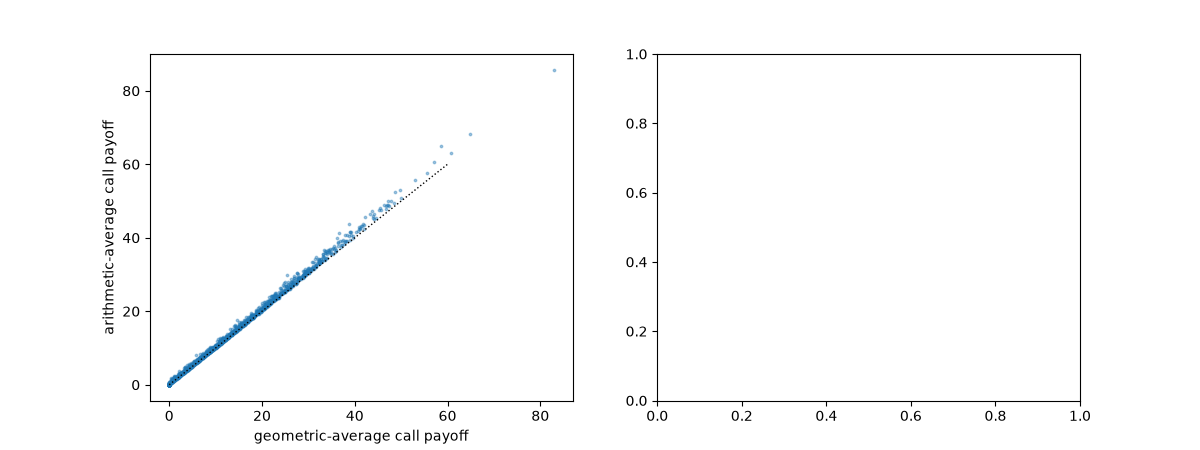
An average-rate option pays on the average price over its life, which makes it cheaper than a vanilla option and harder to manipulate at expiry. Angelien Kemna and Ton Vorst (1990) observed that a geometric average of lognormal prices is lognormal, with volatility \(\sigma/\sqrt3\) under continuous averaging, so its option has a Black-Scholes formula. The arithmetic average traded in practice has none, but the geometric option is so tightly correlated with it that it makes a near-perfect Monte Carlo control variate.

import matplotlib.pyplot as plt
import numpy as np

from financialkit.exotic_options import arithmetic_asian_mc, geometric_asian_price
from financialkit.integrators import gbm_paths
from financialkit.options import black_scholes_price

S, T, r, sigma, n = 100.0, 1.0, 0.05, 0.25, 12

Arithmetic and geometric payoffs on the same paths

_, paths = gbm_paths(S, r, sigma, T, n, 3000, rng=0)
A = paths[:, 1:].mean(axis=1)
G = np.exp(np.log(paths[:, 1:]).mean(axis=1))
fig, axes = plt.subplots(1, 2, figsize=(12, 4.5))
axes[0].scatter(np.maximum(G - 100, 0), np.maximum(A - 100, 0), s=3, alpha=0.4)
axes[0].plot([0, 60], [0, 60], "k:", lw=1)
axes[0].set_xlabel("geometric-average call payoff")
axes[0].set_ylabel("arithmetic-average call payoff")

res = arithmetic_asian_mc(S, 100.0, T, r, sigma, n_fixings=n, n_paths=20_000, rng=2)
print(f"geometric (closed form) {geometric_asian_price(S, 100.0, T, r, sigma, n_fixings=n):.4f}")
print(f"arithmetic: crude {res.crude_estimate:.4f} +/- {res.crude_std_error:.4f}, controlled {res.estimate:.4f} +/- {res.std_error:.4f}")
print(f"R^2 = {res.r_squared:.5f}: variance reduced {1 / (1 - res.r_squared):.0f} times")

geometric (closed form) 6.9907
arithmetic: crude 7.3192 +/- 0.0755, controlled 7.3102 +/- 0.0027
R^2 = 0.99875: variance reduced 801 times

Averaging lowers the price

K = np.linspace(70.0, 130.0, 13)
axes[1].plot(K, black_scholes_price(S, K, T, r, sigma), "k--", label="vanilla call")
axes[1].plot(K, geometric_asian_price(S, K, T, r, sigma), label="geometric, continuous")
arith = [arithmetic_asian_mc(S, k, T, r, sigma, n_fixings=n, n_paths=5_000, rng=2) for k in K]
axes[1].errorbar(K, [a.estimate for a in arith], yerr=[2 * a.std_error for a in arith], fmt="o", ms=4, label=f"arithmetic, {n} fixings (MC)")
axes[1].set_xlabel("strike K")
axes[1].set_ylabel("value")
axes[1].legend()
fig.tight_layout()
plt.show()