Turnbull-Wakeman Asian approximation

Stuart Turnbull and Lee Wakeman (1991) priced the arithmetic average \(A\) as if it were lognormal with the right first two moments: Black’s formula on the forward \(E[A]\) with volatility

\[\sigma_A^2 = \frac{1}{T}\ln\frac{E[A^2]}{E[A]^2}.\]

The moments are exact (Levy’s sums for discrete fixings), only the shape of the distribution is approximated. The approximation is excellent at moderate volatility and drifts as the average’s distribution grows more skewed than a lognormal.

import matplotlib.pyplot as plt
import numpy as np

from financialkit.exotic_options import arithmetic_asian_mc, geometric_asian_price, turnbull_wakeman_price

S, K, T, r, n = 100.0, 100.0, 1.0, 0.05, 12
sigmas = np.array([0.1, 0.2, 0.3, 0.4, 0.5, 0.6])
mc = [arithmetic_asian_mc(S, K, T, r, s, n_fixings=n, n_paths=20_000, rng=3) for s in sigmas]
tw = np.array([turnbull_wakeman_price(S, K, T, r, s, n_fixings=n) for s in sigmas])
geo = geometric_asian_price(S, K, T, r, sigmas, n_fixings=n)

Approximation against controlled Monte Carlo

fig, axes = plt.subplots(1, 2, figsize=(12, 4))
axes[0].plot(sigmas, tw, "s-", label="Turnbull-Wakeman")
axes[0].errorbar(sigmas, [m.estimate for m in mc], yerr=[2 * m.std_error for m in mc], fmt="o", label="Monte Carlo")
axes[0].plot(sigmas, geo, ":", label="geometric (lower bound)")
axes[0].set_xlabel(r"volatility $\sigma$")
axes[0].set_ylabel("at-the-money arithmetic Asian call")
axes[0].legend()
rel = (tw - np.array([m.estimate for m in mc])) / np.array([m.estimate for m in mc])
axes[1].bar(sigmas, 100 * rel, width=0.06)
axes[1].set_xlabel(r"volatility $\sigma$")
axes[1].set_ylabel("relative error (%)")
fig.tight_layout()
for s, t, m in zip(sigmas, tw, mc, strict=True):
    print(f"sigma = {s:.1f}: TW {t:.4f}, MC {m.estimate:.4f} +/- {m.std_error:.4f}")
plt.show()

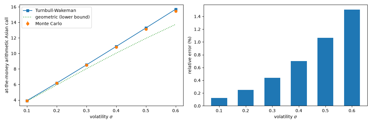
sigma = 0.1: TW 3.9105, MC 3.9056 +/- 0.0005
sigma = 0.2: TW 6.1742, MC 6.1587 +/- 0.0017
sigma = 0.3: TW 8.5178, MC 8.4808 +/- 0.0038
sigma = 0.4: TW 10.8892, MC 10.8133 +/- 0.0069
sigma = 0.5: TW 13.2800, MC 13.1401 +/- 0.0113
sigma = 0.6: TW 15.6890, MC 15.4559 +/- 0.0171