Merton’s down-and-out call

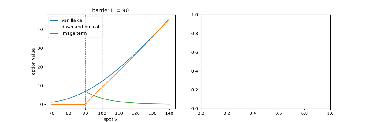
In the paper that put the Black-Scholes model on a rigorous footing, Robert Merton (1973) also priced the first barrier option: a call that dies if the stock falls to \(H\). The barrier is an absorbing boundary for the log-price, and the method of images from the heat equation cancels the probability of crossing it by subtracting a call started from the mirror image \(H^2/S\) of the spot:

\[C_{do} = c(S) - \left(\frac{H}{S}\right)^{2b/\sigma^2 - 1} c\!\left(\frac{H^2}{S}\right).\]

The knock-out is cheaper than the call, and the discount grows as the spot approaches the barrier, where the option is worth nothing.

import matplotlib.pyplot as plt
import numpy as np

from financialkit.exotic_options import barrier_option_mc, merton_down_and_out_call, plot_price_profile
from financialkit.options import black_scholes_price

K, T, r, sigma = 100.0, 1.0, 0.05, 0.25
S = np.linspace(70.0, 140.0, 200)

The call, its image and their difference

H = 90.0
alive = S > H
call = black_scholes_price(S, K, T, r, sigma)
knock_out = merton_down_and_out_call(S, K, H, T, r, sigma)
fig, axes = plt.subplots(1, 2, figsize=(12, 4))
plot_price_profile(
    S, {"vanilla call": call, "down-and-out call": knock_out, "image term": np.where(alive, call - knock_out, np.nan)}, ax=axes[0], markers=(H, K)
)
axes[0].set_title(f"barrier H = {H:g}")

Text(0.5, 1.0, 'barrier H = 90')

Lower barriers cost less

The ratio to the vanilla call rises to one as the barrier moves away. Bridge-corrected Monte Carlo confirms one point on each curve.

for H in (60.0, 75.0, 90.0, 95.0):
    ratio = np.where(S > H, merton_down_and_out_call(S, K, H, T, r, sigma) / call, 0.0)
    axes[1].plot(S, ratio, label=f"H = {H:g}")
    res = barrier_option_mc(110.0, K, H, T, r, sigma, n_steps=25, n_paths=20_000, rng=0)
    axes[1].errorbar(
        110.0,
        res.estimate / black_scholes_price(110.0, K, T, r, sigma),
        yerr=2 * res.std_error / black_scholes_price(110.0, K, T, r, sigma),
        fmt="k.",
        capsize=3,
    )
axes[1].set_xlabel("spot S")
axes[1].set_ylabel("knock-out / vanilla")
axes[1].legend()
fig.tight_layout()
plt.show()