Geske compound options

Robert Geske (1979) priced an option on an option. His motivation was corporate finance: if equity is a call on the firm’s assets, a stock option is a call on a call, and its implied volatility should rise as the stock falls and leverage grows. The compound call is exercised at \(T_1\) only if the underlying option is worth more than the compound strike, which happens above a critical spot \(I\), and the joint law of the price at \(T_1\) and \(T_2\) brings in the bivariate normal distribution with correlation \(\sqrt{T_1/T_2}\).

import matplotlib.pyplot as plt
import numpy as np

from financialkit.exotic_options import compound_option_price, critical_price
from financialkit.options import black_scholes_price

K1, K2, T1, T2, r, sigma = 5.0, 100.0, 0.25, 1.0, 0.05, 0.3
S = np.linspace(60.0, 150.0, 200)
print(f"Haug (2007), 4.6, put on call: {compound_option_price(500.0, 50.0, 520.0, 0.25, 0.5, 0.08, 0.35, q=0.03, option_type='put'):.4f}")

Haug (2007), 4.6, put on call: 21.1964

The four compound options

fig, axes = plt.subplots(1, 2, figsize=(12, 4))
for underlying in ("call", "put"):
    I = critical_price(K1, K2, T2 - T1, r, sigma, underlying_type=underlying)
    for option_type in ("call", "put"):
        axes[0].plot(
            S, compound_option_price(S, K1, K2, T1, T2, r, sigma, option_type=option_type, underlying_type=underlying), label=f"{option_type} on {underlying}"
        )
    axes[0].axvline(I, color="C0" if underlying == "call" else "C2", ls=":", lw=1)
axes[0].set_xlabel("spot S (dotted: critical spots I)")
axes[0].set_ylabel("value")
axes[0].legend()

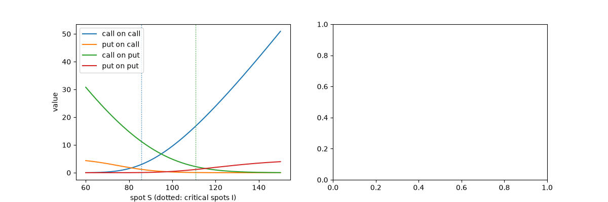
<matplotlib.legend.Legend object at 0x116f13cb0>

Compound put-call parity

Call on call minus put on call is the call minus the discounted compound strike, whatever the spot.

cc = compound_option_price(S, K1, K2, T1, T2, r, sigma)
pc = compound_option_price(S, K1, K2, T1, T2, r, sigma, option_type="put")
axes[1].plot(S, cc - pc, lw=3, label="call on call - put on call")
axes[1].plot(S, black_scholes_price(S, K2, T2, r, sigma) - K1 * np.exp(-r * T1), "k--", label=r"$c(S) - K_1 e^{-rT_1}$")
axes[1].set_xlabel("spot S")
axes[1].legend()
fig.tight_layout()
plt.show()