Ho and Stoll: the dealer’s inventory problem

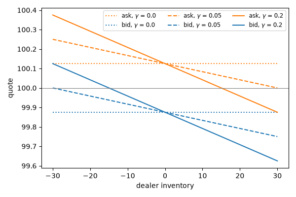
Thomas Ho and Hans Stoll (1981) gave the dealer risk aversion. Holding inventory exposes it to price moves, so a dealer who is long lowers both quotes, making a sale to it less attractive and a purchase from it more so, until the inventory returns to zero. With order arrivals \(\lambda = \alpha - \beta\delta\) on each side, the spread itself, \(\alpha/\beta\), does not depend on the inventory: only its position does.

import matplotlib.pyplot as plt
import numpy as np

from financialkit.market_microstructure import ho_stoll_quotes

alpha, beta, sigma = 10.0, 40.0, 0.5
inventory = np.linspace(-30, 30, 61)

Quotes shade against inventory

fig, ax = plt.subplots(figsize=(6, 4))
for g, ls in [(0.0, ":"), (0.05, "--"), (0.2, "-")]:
    b, a = ho_stoll_quotes(100.0, inventory, alpha, beta, g, sigma)
    ax.plot(inventory, a, "C1" + ls, label=f"ask, $\\gamma$ = {g}")
    ax.plot(inventory, b, "C0" + ls, label=f"bid, $\\gamma$ = {g}")
ax.axhline(100.0, color="0.5", lw=0.8)
ax.set_xlabel("dealer inventory")
ax.set_ylabel("quote")
ax.legend(ncol=3, fontsize="small")
fig.tight_layout()

Inventory control in action

Each period, buy and sell orders arrive as Poisson counts at the rates the quotes imply. A risk-neutral dealer’s inventory wanders like a random walk; the risk-averse dealer’s is mean-reverting.

rng = np.random.default_rng(4)
n_paths, n_periods = 400, 300
paths = {}
for g in (0.0, 0.2):
    I = np.zeros((n_paths, n_periods + 1))
    for t in range(n_periods):
        b, a = ho_stoll_quotes(100.0, I[:, t], alpha, beta, g, sigma)
        lam_a = np.clip(alpha - beta * (a - 100.0), 0, None)
        lam_b = np.clip(alpha - beta * (100.0 - b), 0, None)
        I[:, t + 1] = I[:, t] - rng.poisson(lam_a) + rng.poisson(lam_b)
    paths[g] = I
    print(f"gamma = {g}: inventory sd after {n_periods} periods {I[:, -1].std():.1f}")

fig, ax = plt.subplots(figsize=(7, 3.5))
for g, color in [(0.0, "C3"), (0.2, "C0")]:
    ax.plot(paths[g][:10].T, color=color, lw=0.7, alpha=0.7)
    ax.plot([], [], color=color, label=f"$\\gamma$ = {g}")
ax.set_xlabel("period")
ax.set_ylabel("inventory")
ax.legend()
fig.tight_layout()

plt.show()

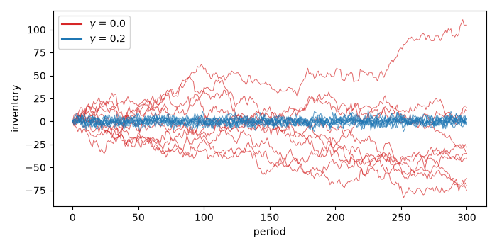
gamma = 0.0: inventory sd after 300 periods 53.6
gamma = 0.2: inventory sd after 300 periods 3.5