Demsetz: the bid-ask spread as the price of immediacy

Harold Demsetz (1968) argued that a trader who wants to trade now pays the dealer the spread for standing ready, and that the spread shrinks as trading activity grows, because a busy dealer turns over inventory faster. Today the spread is measured three ways: the quoted spread on the screen, the effective spread actually paid relative to the midquote, and the realized spread the liquidity provider keeps once the price has moved; the difference is the price impact, lost to better-informed traders.

import matplotlib.pyplot as plt
import numpy as np

from financialkit.market_microstructure import effective_spread, price_impact, quoted_spread, realized_spread
from financialkit.market_microstructure.visualizers import plot_quotes

rng = np.random.default_rng(0)

Quoted, effective and realized spreads

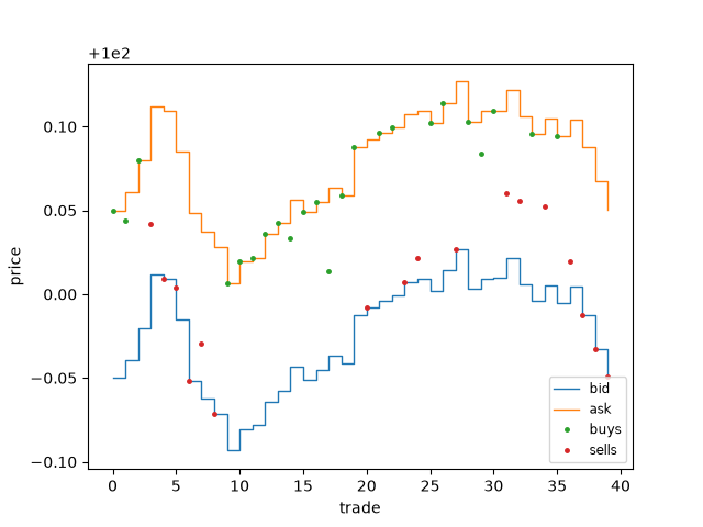
A dealer quotes 10 cents wide around the efficient price. Trades fill at the quotes or, sometimes, inside them; each trade then moves the efficient price by a cent in its own direction (information) plus noise.

n, half, impact = 2000, 0.05, 0.01
side = rng.choice([-1.0, 1.0], n)
m = 100 + np.cumsum(impact * side + 0.01 * rng.standard_normal(n))
mid = np.concatenate([[100.0], m[:-1]])  # the quote before each trade
bid, ask = mid - half, mid + half
price = mid + side * np.where(rng.random(n) < 0.3, rng.uniform(0, half, n), half)
later = np.concatenate([m[5:], np.full(5, m[-1])])  # midquote five trades later

for name, x in [
    ("quoted", quoted_spread(bid, ask)),
    ("effective", effective_spread(price, bid, ask, side)),
    ("realized", realized_spread(price, later, side)),
    ("price impact", price_impact(bid, ask, later, side)),
]:
    print(f"{name:13s} {x.mean():.4f}")

plot_quotes(price[:40], bid[:40], ask[:40], side=side[:40])

quoted        0.1000
effective     0.0843
realized      0.0649
price impact  0.0194

<Axes: xlabel='trade', ylabel='price'>

Demsetz’s cross-section

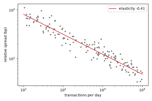
Demsetz regressed the spreads of 192 NYSE stocks on their number of transactions and found a strongly negative slope. Here a synthetic cross-section with an elasticity of -0.4 is recovered by a log-log fit.

trades_per_day = 10 ** rng.uniform(1, 4, 150)
rel_spread = 0.02 * trades_per_day**-0.4 * np.exp(0.25 * rng.standard_normal(150))
slope, intercept = np.polyfit(np.log(trades_per_day), np.log(rel_spread), 1)
fig, ax = plt.subplots(figsize=(6, 4))
ax.loglog(trades_per_day, 1e4 * rel_spread, ".", color="0.5")
grid = np.logspace(1, 4, 50)
ax.loglog(grid, 1e4 * np.exp(intercept) * grid**slope, "C3", label=f"elasticity {slope:.2f}")
ax.set_xlabel("transactions per day")
ax.set_ylabel("relative spread (bp)")
ax.legend()
fig.tight_layout()

plt.show()