Brennan-Schwartz American put

Michael Brennan and Eduardo Schwartz (1977) priced the American put with an implicit scheme and a direct solve: eliminate the tridiagonal system starting from the top of the grid, then substitute back upward from \(S = 0\), taking the larger of the computed value and the payoff at each node. Because the put is exercised on a single interval at the bottom of the grid, this one pass solves the complementarity problem exactly. brennan_schwartz() matches PSOR to rounding at a fraction of the cost.

import time

import matplotlib.pyplot as plt
import numpy as np

from financialkit.options import CRRTree
from financialkit.pde_methods import CrankNicolson

S, K, T, r, sigma = 50.0, 50.0, 5 / 12, 0.10, 0.40
tree = CRRTree(2000).price(S, K, T, r, sigma, option_type="put", american=True).price
for method in ("brennan_schwartz", "psor"):
    t0 = time.perf_counter()
    res = CrankNicolson(400, 200, rannacher_steps=2, american_method=method).price(S, K, T, r, sigma, option_type="put", american=True)
    print(f"{method:16s} {res.price:.6f} in {time.perf_counter() - t0:.3f} s, {res.lcp_iterations} iterations")
print(f"CRR tree         {tree:.6f}")

brennan_schwartz 4.282866 in 0.128 s, 202 iterations
psor             4.282866 in 0.015 s, 3606 iterations
CRR tree         4.283922

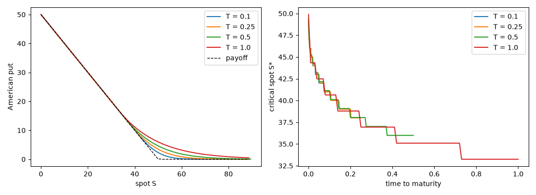
The put across spots and maturities

maturities = [0.1, 0.25, 0.5, 1.0]
fig, axes = plt.subplots(1, 2, figsize=(11, 4))
for T_ in maturities:
    res = CrankNicolson(200, 100, rannacher_steps=2, american_method="brennan_schwartz").price(S, K, T_, r, sigma, option_type="put", american=True)
    near = res.S < 90
    axes[0].plot(res.S[near], res.V[near], label=f"T = {T_}")
    axes[1].plot(T_ - res.times, res.exercise_boundary, label=f"T = {T_}")
axes[0].plot(res.S[near], np.maximum(K - res.S[near], 0.0), "k--", lw=1, label="payoff")
axes[0].set_xlabel("spot S")
axes[0].set_ylabel("American put")
axes[0].legend()
axes[1].set_xlabel("time to maturity")
axes[1].set_ylabel("critical spot S*")
axes[1].legend()
fig.tight_layout()
plt.show()