Forsyth-Vetzal penalty method

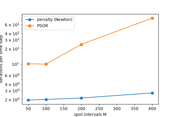
Peter Forsyth and Kenneth Vetzal (2002) replaced the complementarity constraint by a penalty: on nodes where the value falls below the payoff, add \(\rho\,(g - x)\) with a large \(\rho\). The resulting nonlinear system is solved by a Newton (policy) iteration that only changes which nodes are penalised, and converges in two or three tridiagonal solves per time step, independently of the grid size – unlike PSOR, whose sweep count grows as the grid is refined. penalty_solve() implements it.

import matplotlib.pyplot as plt
import numpy as np

from financialkit.pde_methods import CrankNicolson

S, K, T, r, sigma = 100.0, 100.0, 1.0, 0.06, 0.3
ms = np.array([50, 100, 200, 400])
iters = {"penalty": [], "psor": []}
prices = {"penalty": [], "psor": []}
for m in ms:
    for method in iters:
        res = CrankNicolson(m, 50, rannacher_steps=2, american_method=method).price(S, K, T, r, sigma, option_type="put", american=True)
        iters[method].append(res.lcp_iterations / 54)  # 50 steps, two of them as four half steps
        prices[method].append(res.price)
for m, a, b in zip(ms, prices["penalty"], prices["psor"], strict=True):
    print(f"M = {m:3d}: penalty {a:.6f}, PSOR {b:.6f}")

M =  50: penalty 9.432503, PSOR 9.432503
M = 100: penalty 9.510534, PSOR 9.510534
M = 200: penalty 9.523474, PSOR 9.523474
M = 400: penalty 9.526267, PSOR 9.526266

Iterations per time step as the grid is refined

fig, ax = plt.subplots(figsize=(6, 4))
ax.semilogy(ms, iters["penalty"], "o-", label="penalty (Newton)")
ax.semilogy(ms, iters["psor"], "s-", label="PSOR")
ax.set_xlabel("spot intervals M")
ax.set_ylabel("iterations per time step")
ax.legend()
plt.show()