Sharpe’s single-index model

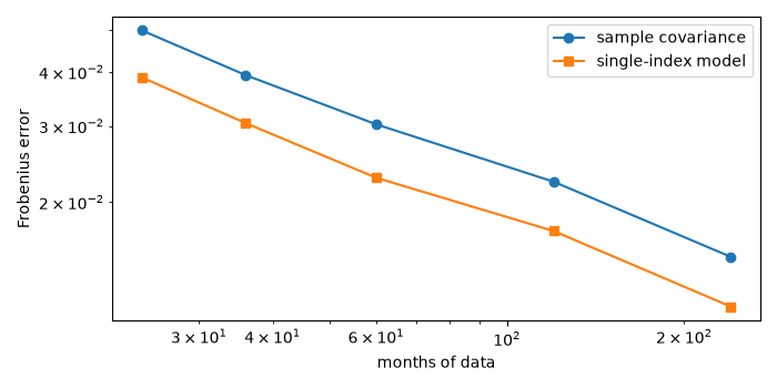
Markowitz’s method needed every pairwise covariance, \(d(d+1)/2\) numbers, which no 1960s computer (or analyst) could supply for hundreds of stocks. William Sharpe (1963) assumed that stocks move together only through a common market index, \(R_i = \alpha_i + \beta_i R_m + \varepsilon_i\), so the covariance is \(\sigma_m^2\beta\beta' + \mathrm{diag}(\sigma_{\varepsilon}^2)\), with \(3d + 1\) parameters. The structure also filters noise: with short histories, the single-index estimate is closer to the truth than the sample covariance.

import matplotlib.pyplot as plt
import numpy as np

from financialkit.portfolio import sample_covariance, single_index_covariance

rng = np.random.default_rng(5)
d, n = 30, 36
beta = rng.uniform(0.5, 1.5, d)
resid = rng.uniform(0.04, 0.10, d)
sig_m = 0.045
true = sig_m**2 * np.outer(beta, beta) + np.diag(resid**2)


def simulate(n_months):
    m = sig_m * rng.standard_normal(n_months)
    return np.outer(m, beta) + resid * rng.standard_normal((n_months, d)), m

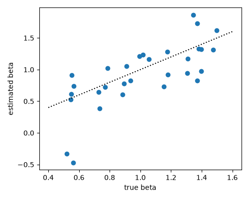
Fitted betas from three years of monthly data

X, m = simulate(n)
si = single_index_covariance(X, m)
fig, ax = plt.subplots(figsize=(5, 4))
ax.plot(beta, si.betas, "o")
ax.plot([0.4, 1.6], [0.4, 1.6], "k:")
ax.set_xlabel("true beta")
ax.set_ylabel("estimated beta")
fig.tight_layout()
print(f"parameters: sample {sample_covariance(X).n_params}, single index {si.n_params}")

parameters: sample 465, single index 91

Estimation error against the length of history

months = [24, 36, 60, 120, 240]
err_s, err_si = [], []
for T in months:
    es, esi = [], []
    for _ in range(30):
        X, m = simulate(T)
        es.append(np.linalg.norm(sample_covariance(X).cov - true))
        esi.append(np.linalg.norm(single_index_covariance(X, m).cov - true))
    err_s.append(np.mean(es))
    err_si.append(np.mean(esi))
fig, ax = plt.subplots(figsize=(7, 3.5))
ax.loglog(months, err_s, "o-", label="sample covariance")
ax.loglog(months, err_si, "s-", label="single-index model")
ax.set_xlabel("months of data")
ax.set_ylabel("Frobenius error")
ax.legend()
fig.tight_layout()
plt.show()