Ledoit-Wolf shrinkage

When the number of assets is comparable to the number of observations, the sample covariance’s eigenvalues spread out far more than the true ones: the smallest are too small, so the minimum-variance optimizer loads up on spurious “riskless” combinations. Olivier Ledoit and Michael Wolf (2004) shrank the sample matrix towards a structured target, \(\delta F + (1 - \delta)S\), with the intensity \(\delta\) estimated from the data to minimize the expected squared error. Their two targets are a scaled identity and the constant-correlation matrix.

import matplotlib.pyplot as plt
import numpy as np

from financialkit.portfolio import ledoit_wolf, min_variance_portfolio, sample_covariance

rng = np.random.default_rng(6)
d = 40
vol = rng.uniform(0.04, 0.1, d)
true = (0.3 + 0.7 * np.eye(d)) * np.outer(vol, vol)
L = np.linalg.cholesky(true)

Eigenvalue dispersion with 60 observations

X = rng.standard_normal((60, d)) @ L.T
S, lw = sample_covariance(X), ledoit_wolf(X, "constant_correlation")
fig, ax = plt.subplots(figsize=(7, 3.5))
for C, label in [(true, "true"), (S.cov, "sample"), (lw.cov, f"Ledoit-Wolf, delta = {lw.shrinkage:.2f}")]:
    ax.semilogy(np.sort(np.linalg.eigvalsh(C))[::-1], "o-", ms=3, label=label)
ax.set_xlabel("eigenvalue rank")
ax.set_ylabel("eigenvalue")
ax.legend()
fig.tight_layout()
print(f"condition numbers: sample {S.condition_number:.0f}, shrunk {lw.condition_number:.0f}")

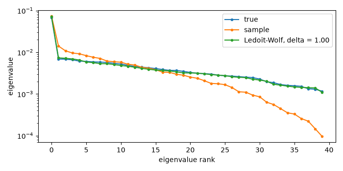
condition numbers: sample 761, shrunk 65

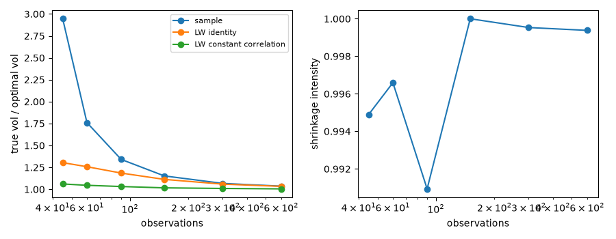
Shrinkage intensity and out-of-sample risk

The true volatility of the minimum-variance portfolio built from each estimate. Shrinkage helps most when data are scarce and fades as they accumulate.

ns = [45, 60, 90, 150, 300, 600]
rows = []
for n in ns:
    r = []
    for _ in range(20):
        X = rng.standard_normal((n, d)) @ L.T
        ests = [sample_covariance(X), ledoit_wolf(X), ledoit_wolf(X, "constant_correlation")]
        r.append([np.sqrt(w @ true @ w) for w in (min_variance_portfolio(e.cov).weights for e in ests)] + [ests[2].shrinkage])
    rows.append(np.mean(r, axis=0))
rows = np.array(rows)
best = min_variance_portfolio(true).volatility
fig, (ax1, ax2) = plt.subplots(1, 2, figsize=(9, 3.5))
for k, label in enumerate(["sample", "LW identity", "LW constant correlation"]):
    ax1.plot(ns, rows[:, k] / best, "o-", label=label)
ax1.set_xscale("log")
ax1.set_xlabel("observations")
ax1.set_ylabel("true vol / optimal vol")
ax1.legend(fontsize=8)
ax2.plot(ns, rows[:, 3], "o-")
ax2.set_xscale("log")
ax2.set_xlabel("observations")
ax2.set_ylabel("shrinkage intensity")
fig.tight_layout()
plt.show()