Merton’s portfolio problem

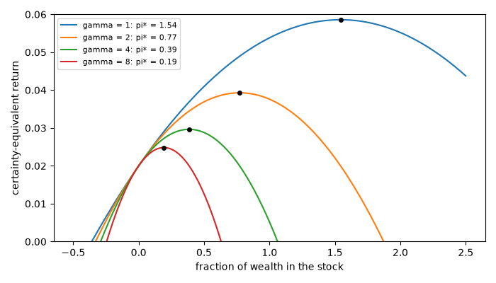
Robert Merton (1969) solved the lifetime consumption and investment problem in continuous time. With a stock following geometric Brownian motion, a riskless rate \(r\) and constant relative risk aversion \(\gamma\), the optimal policy is to keep the constant fraction

\[\pi^* = \frac{\mu - r}{\gamma\sigma^2}\]

of wealth in the stock, rebalancing continuously, and to consume a constant fraction of wealth. The Kelly rule is the case \(\gamma = 1\).

import matplotlib.pyplot as plt
import numpy as np

from financialkit.portfolio import merton_certainty_equivalent, merton_consumption_rate, merton_fraction, merton_wealth_paths

mu, r, sigma = 0.07, 0.02, 0.18

The certainty-equivalent return of each constant mix

pi = np.linspace(-0.5, 2.5, 300)
fig, ax = plt.subplots(figsize=(7, 4))
for gamma in [1.0, 2.0, 4.0, 8.0]:
    star = merton_fraction(mu, r, sigma, gamma)
    ax.plot(pi, merton_certainty_equivalent(pi, mu, r, sigma, gamma), label=f"gamma = {gamma:g}: pi* = {star:.2f}")
    ax.plot(star, merton_certainty_equivalent(star, mu, r, sigma, gamma), "ko", ms=4)
ax.set_ylim(0.0, 0.06)
ax.set_xlabel("fraction of wealth in the stock")
ax.set_ylabel("certainty-equivalent return")
ax.legend(fontsize=8)
fig.tight_layout()
for gamma in [2.0, 4.0]:
    print(f"gamma = {gamma:g}: consume {merton_consumption_rate(mu, r, sigma, gamma, 0.03):.2%} of wealth a year")

gamma = 2: consume 3.46% of wealth a year
gamma = 4: consume 2.97% of wealth a year

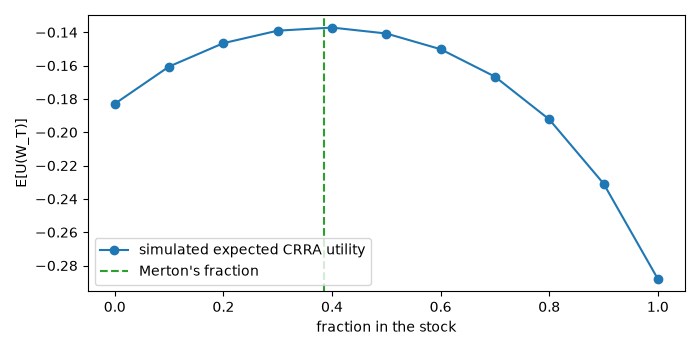
Monte Carlo check: no other mix gives a higher expected utility

Terminal wealth after 10 years for \(\gamma = 4\), simulated exactly through financialkit.integrators.gbm_paths() on common random numbers.

gamma, T = 4.0, 10.0
mixes = np.linspace(0.0, 1.0, 11)
eu = []
for m in mixes:
    # The same seed for every mix: common random numbers.
    _, W = merton_wealth_paths(m, mu, r, sigma, T, 1, 100_000, rng=0)
    eu.append(np.mean(W[:, -1] ** (1 - gamma)) / (1 - gamma))
fig, ax = plt.subplots(figsize=(7, 3.5))
ax.plot(mixes, eu, "o-", label="simulated expected CRRA utility")
ax.axvline(merton_fraction(mu, r, sigma, gamma), color="C2", ls="--", label="Merton's fraction")
ax.set_xlabel("fraction in the stock")
ax.set_ylabel("E[U(W_T)]")
ax.legend()
fig.tight_layout()
plt.show()