Sklar’s theorem and the Gaussian copula

Sklar (1959) showed that every joint distribution is its marginals glued together by a copula \(C\):

\[F(x_1, x_2) = C\big(F_1(x_1), F_2(x_2)\big).\]

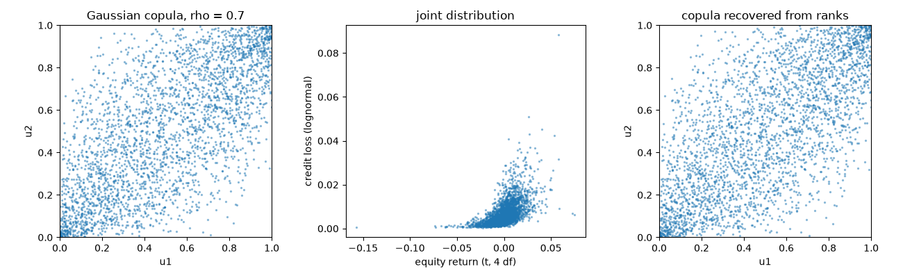
Risk managers can therefore model each asset’s return on its own and choose the dependence separately. Here a Gaussian copula with correlation 0.7 joins a fat-tailed Student-t equity return to a skewed credit loss, and the copula is recovered from the joint sample by ranks alone.

import matplotlib.pyplot as plt
import numpy as np
from scipy import stats

from financialkit.risk import apply_marginals, copula_kendall_tau, gaussian_copula_sample, pseudo_observations
from financialkit.risk.visualizers import plot_copula

corr = np.array([[1.0, 0.7], [0.7, 1.0]])
u = gaussian_copula_sample(corr, 3000, rng=0)

One copula, any marginals

equity = stats.t(4, scale=0.01)
credit = stats.lognorm(0.8, scale=0.005)
x = apply_marginals(u, [equity.ppf, credit.ppf])

fig, axes = plt.subplots(1, 3, figsize=(13, 4))
plot_copula(u, ax=axes[0], title="Gaussian copula, rho = 0.7")
axes[1].scatter(x[:, 0], x[:, 1], s=2, alpha=0.4)
axes[1].set_xlabel("equity return (t, 4 df)")
axes[1].set_ylabel("credit loss (lognormal)")
axes[1].set_title("joint distribution")
plot_copula(pseudo_observations(x), ax=axes[2], title="copula recovered from ranks")
fig.tight_layout()

Rank correlation is a property of the copula

Pearson correlation changes with the marginals; Kendall’s tau does not, and for the Gaussian copula it equals \(\tfrac{2}{\pi}\arcsin\rho\).

print(f"Pearson, uniforms {np.corrcoef(u.T)[0, 1]:.3f}  vs  Pearson, t/lognormal {np.corrcoef(x.T)[0, 1]:.3f}")
print(f"Kendall, uniforms {stats.kendalltau(*u.T).statistic:.3f}  vs  Kendall, t/lognormal {stats.kendalltau(*x.T).statistic:.3f}")
print(f"theory 2/pi arcsin(0.7) = {copula_kendall_tau(0.7):.3f}")

plt.show()

Pearson, uniforms 0.677  vs  Pearson, t/lognormal 0.570
Kendall, uniforms 0.486  vs  Kendall, t/lognormal 0.486
theory 2/pi arcsin(0.7) = 0.494