Fisher-Tippett: the three laws of the maximum

Fisher and Tippett (1928) proved that the largest of \(n\) i.i.d. losses, once centred and scaled, can converge to only three limits: Fréchet for power-law tails, Gumbel for exponential-type tails and Weibull for bounded ones. They are the generalized extreme value law

\[H_\xi(x) = \exp\left(-(1 + \xi x)^{-1/\xi}\right),\]

with shape \(\xi > 0\), \(= 0\) and \(< 0\). Fitting it to the worst loss of each month tells us which family a return series belongs to, and extrapolates to crashes rarer than any in the sample.

import matplotlib.pyplot as plt
import numpy as np
from scipy import stats

from financialkit.risk import fit_gev, gev_return_level
from financialkit.risk.visualizers import plot_gev_fit

rng = np.random.default_rng(0)
n_months, days = 600, 21

Three parents, three limits

Student-t losses (3 degrees of freedom) have a power tail, normal losses a Gaussian one, and uniform losses stop at a bound. The fitted shapes are positive, near zero and near -1. Convergence to the limit is slow: monthly maxima of t(3) losses give a shape below the asymptotic \(1/\nu = 1/3\), and normal maxima a slightly negative one.

parents = {
    "Student-t(3): Fréchet": stats.t(3).rvs(size=n_months * days, random_state=rng),
    "normal: Gumbel": rng.standard_normal(n_months * days),
    "uniform: Weibull": rng.uniform(-1, 1, n_months * days),
}
fig, axes = plt.subplots(1, 3, figsize=(12, 3.8))
for ax, (name, losses) in zip(axes, parents.items(), strict=True):
    fit = fit_gev(-losses, days)
    plot_gev_fit(fit, ax=ax)
    ax.set_title(name)
    print(f"{name:24s} xi = {fit.xi:+.3f}")
fig.tight_layout()

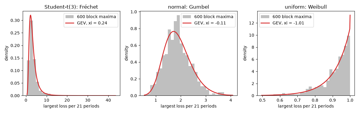
Student-t(3): Fréchet    xi = +0.236
normal: Gumbel           xi = -0.112
uniform: Weibull         xi = -1.005

Return levels of a fat-tailed market

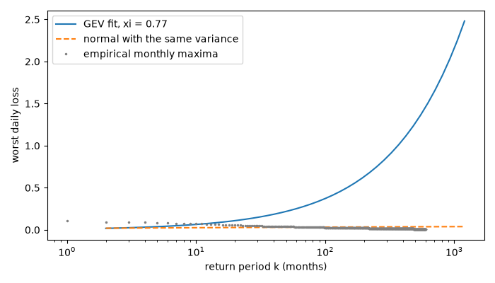
The “once in k months” worst daily loss. For the Fréchet fit it grows like a power of \(k\), far faster than the normal fit would suggest for the same data.

returns = 0.01 * stats.t(3).rvs(size=n_months * days, random_state=rng) / np.sqrt(3.0)
fit = fit_gev(returns, days)
k = np.geomspace(2, 1200, 50)
mu, sd = returns.mean(), returns.std()
normal_level = -(mu + sd * stats.norm.ppf(1 / (k * days)))

fig, ax = plt.subplots(figsize=(7, 4))
ax.semilogx(k, gev_return_level(fit, k), label=f"GEV fit, xi = {fit.xi:.2f}")
ax.semilogx(k, normal_level, "--", label="normal with the same variance")
ax.plot(np.arange(1, n_months + 1)[::-1] * 1.0, np.sort(fit.maxima), ".", color="0.5", ms=3, label="empirical monthly maxima")
ax.set_xlabel("return period k (months)")
ax.set_ylabel("worst daily loss")
ax.legend()
fig.tight_layout()

plt.show()