Hull and White’s stochastic volatility

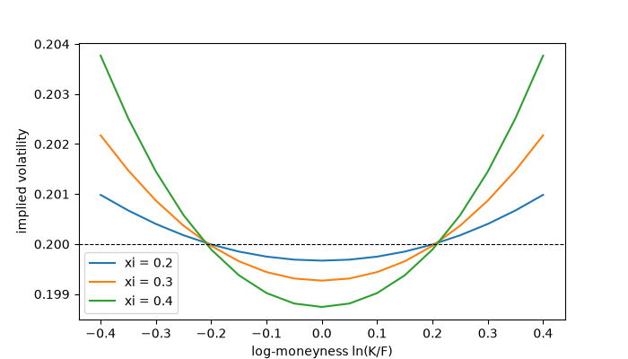
Hull and White (1987) let the variance follow its own lognormal diffusion, \(dV = \xi V\,dW\), independent of the stock. Conditional on the variance path the stock is lognormal with the path’s average variance \(\bar V\), so the option price is the Black-Scholes price averaged over the distribution of \(\bar V\): the mixing formula. They expanded it in a series in \(\xi^2 T\); here it is also computed by simulating variance paths. Because the variance is uncorrelated with the stock the smile is symmetric, and the at-the-money price falls below Black-Scholes, which is concave in the variance there.

import matplotlib.pyplot as plt
import numpy as np

from financialkit.options import black_scholes_price, implied_volatility
from financialkit.stochastic_volatility import hull_white_mixing_mc, hull_white_price
from financialkit.stochastic_volatility.visualizers import plot_smile

S, T, r, sigma0 = 100.0, 1.0, 0.0, 0.2

Series against mixing Monte Carlo

The series is accurate while \(\xi^2 T\) is small and drifts away as it grows; the mixing Monte Carlo has no such limit.

bs = black_scholes_price(S, 100.0, T, r, sigma0)
print(f"Black-Scholes at sigma0: {bs:.4f}")
print("   xi   series   mixing MC  (+/- 2 se)")
for xi in (0.2, 0.4, 0.8, 1.2):
    mc = hull_white_mixing_mc(S, 100.0, T, r, sigma0, xi, n_paths=20_000, rng=0)
    print(f"{xi:5.1f} {hull_white_price(S, 100.0, T, r, sigma0, xi):8.4f}   {mc.estimate:8.4f}   {2 * mc.std_error:.4f}")

Black-Scholes at sigma0: 7.9656
   xi   series   mixing MC  (+/- 2 se)
  0.2   7.9524     7.9566   0.0065
  0.4   7.9156     7.9214   0.0130
  0.8   7.8466     7.7753   0.0256
  1.2   8.6741     7.5371   0.0377

The symmetric smile

F = S * np.exp(r * T)
K = F * np.exp(np.linspace(-0.4, 0.4, 17))
fig, ax = plt.subplots(figsize=(7, 4))
for xi in (0.2, 0.3, 0.4):
    vols = implied_volatility(hull_white_price(S, K, T, r, sigma0, xi), S, K, T, r)
    plot_smile(K, vols, forward=F, ax=ax, label=f"xi = {xi}")
ax.axhline(sigma0, color="k", lw=0.8, ls="--")

plt.show()