The Heston model

Steven Heston (1993) gave the variance a mean-reverting square-root diffusion correlated with the stock,

\[dS = r S\,dt + \sqrt{v} S\,dW_1, \qquad dv = \kappa(\theta - v)\,dt + \xi\sqrt{v}\,dW_2, \qquad dW_1 dW_2 = \rho\,dt,\]

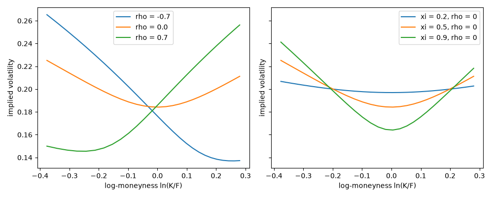
and found its characteristic function in closed form. The call is \(S P_1 - K e^{-rT} P_2\), with each exercise probability a single Fourier integral. A negative correlation, the stock falling as volatility rises, produces the equity skew; the volatility of variance \(\xi\) produces the curvature.

import matplotlib.pyplot as plt
import numpy as np

from financialkit.stochastic_volatility import HestonModel, heston_paths, heston_price
from financialkit.stochastic_volatility.visualizers import plot_heston_paths, plot_smile

S, T, r = 100.0, 1.0, 0.02
base = dict(v0=0.04, kappa=1.5, theta=0.04, xi=0.5)

m = HestonModel(rho=-0.7, **base)
print("Feller condition 2 kappa theta >= xi^2:", m.feller_satisfied)
print(f"at-the-money call by Heston's two probabilities: {heston_price(m, S, 100.0, T, r):.4f}")

plot_heston_paths(heston_paths(m, S, T, r, n_steps=250, n_paths=10, rng=0))

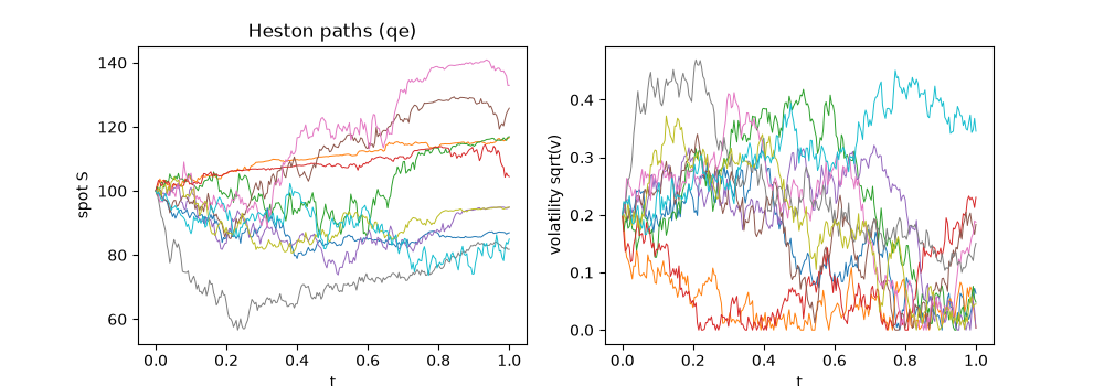
Feller condition 2 kappa theta >= xi^2: False
at-the-money call by Heston's two probabilities: 8.1950

array([<Axes: title={'center': 'Heston paths (qe)'}, xlabel='t', ylabel='spot S'>,
       <Axes: xlabel='t', ylabel='volatility sqrt(v)'>], dtype=object)

Correlation sets the skew, vol of vol the curvature

K = np.linspace(70, 135, 27)
F = S * np.exp(r * T)
fig, (ax1, ax2) = plt.subplots(1, 2, figsize=(10, 4), sharey=True)
for rho in (-0.7, 0.0, 0.7):
    plot_smile(K, HestonModel(rho=rho, **base).implied_vol(S, K, T, r), forward=F, ax=ax1, label=f"rho = {rho}")
for xi in (0.2, 0.5, 0.9):
    plot_smile(K, HestonModel(0.04, 1.5, 0.04, xi, 0.0).implied_vol(S, K, T, r), forward=F, ax=ax2, label=f"xi = {xi}, rho = 0")
fig.tight_layout()

plt.show()