Cox’s constant elasticity of variance

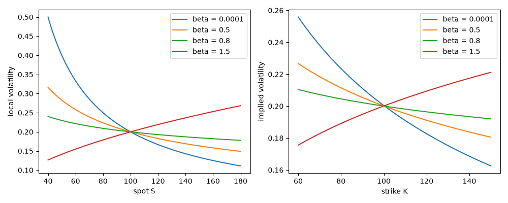
In 1975 John Cox let the volatility depend on the price, \(dS = r S\,dt + \sigma S^{\beta}\,dW\). The local volatility is \(\sigma S^{\beta - 1}\): for \(\beta < 1\) it rises as the price falls, the leverage effect Fischer Black had just documented, and the implied volatility skews down in the strike. Schroder (1989) gave the prices in closed form with the noncentral chi-square distribution. Here the closed form is checked against an Euler simulation of the SDE and the skew is shown for several elasticities, each scaled to a 20% at-the-money local volatility.

import matplotlib.pyplot as plt
import numpy as np

from financialkit.integrators import euler_maruyama, njit
from financialkit.options import implied_volatility
from financialkit.stochastic_volatility import cev_local_vol, cev_price
from financialkit.stochastic_volatility.visualizers import plot_smile

S, T, r = 100.0, 1.0, 0.03

Closed form against simulation

@njit
def drift(x, t, p):
    return p[0] * x


@njit
def diffusion(x, t, p):
    return p[1] * np.maximum(x, 0.0) ** p[2]


beta = 0.5
sigma = 0.2 * S ** (1 - beta)
_, paths = euler_maruyama(drift, diffusion, S, T, 100, 20_000, params=[r, sigma, beta], rng=0)
for K in (80.0, 100.0, 120.0):
    pay = np.exp(-r * T) * np.maximum(paths[:, -1] - K, 0.0)
    print(f"K = {K:5.0f}: Schroder {cev_price(S, K, T, r, sigma, beta):.4f}, Euler MC {pay.mean():.4f} +/- {2 * pay.std() / np.sqrt(pay.size):.4f}")

K =    80: Schroder 23.4115, Euler MC 23.5832 +/- 0.2600
K =   100: Schroder 9.4167, Euler MC 9.5563 +/- 0.1902
K =   120: Schroder 2.4856, Euler MC 2.5879 +/- 0.1011

The skew

K = np.linspace(60, 150, 31)
fig, (ax1, ax2) = plt.subplots(1, 2, figsize=(10, 4))
grid = np.linspace(40, 180, 100)
for beta in (0.0001, 0.5, 0.8, 1.5):
    sigma = 0.2 * S ** (1 - beta)
    ax1.plot(grid, cev_local_vol(grid, sigma, beta), label=f"beta = {beta:g}")
    vols = implied_volatility(cev_price(S, K, T, r, sigma, beta), S, K, T, r)
    plot_smile(K, vols, ax=ax2, label=f"beta = {beta:g}")
ax1.set_xlabel("spot S")
ax1.set_ylabel("local volatility")
ax1.legend()
fig.tight_layout()

plt.show()