Dupire’s local volatility

In 1994 Bruno Dupire showed that a full surface of call prices \(C(K, T)\) pins down a unique local volatility \(\sigma(S, t)\) that reproduces it,

\[\sigma^2(K, T) = \frac{\partial_T C + r K\,\partial_K C}{\tfrac12 K^2\,\partial_{KK} C},\]

the forward equation of the option price read backwards. Here the prices come from Cox’s CEV model, whose local volatility \(\sigma S^{\beta - 1}\) is known, so finite differences of the price grid can be checked against it. Simulating the recovered diffusion then reprices the options.

import matplotlib.pyplot as plt
import numpy as np

from financialkit.stochastic_volatility import cev_local_vol, cev_price, dupire_local_vol, local_vol_paths
from financialkit.stochastic_volatility.visualizers import plot_local_vol

S, r, beta, sigma = 100.0, 0.03, 0.5, 2.5
K = np.linspace(50, 180, 131)
T = np.linspace(0.25, 1.5, 51)
C = cev_price(S, K[None, :], T[:, None], r, sigma, beta)

lv = dupire_local_vol(K, T, C, r)
true = cev_local_vol(K, sigma, beta)
# The first maturity row uses one-sided differences in T, which are least accurate in the wings.
inner = (K > 60) & (K < 160)
print("max |Dupire - CEV| for 60 < K < 160, T > 0.25:", f"{np.nanmax(np.abs(lv.vol[1:, inner] - true[inner])):.1e}")

fig, ax = plt.subplots(figsize=(7, 4))
plot_local_vol(lv, maturities=[0.5, 1.0, 1.5], ax=ax)
ax.plot(K, true, "k--", lw=1, label="CEV: sigma S^(beta - 1)")
ax.set_ylim(0.1, 0.4)
ax.legend()

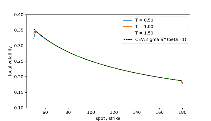
max |Dupire - CEV| for 60 < K < 160, T > 0.25: 3.7e-03

<matplotlib.legend.Legend object at 0x1172b4050>

Repricing by simulation

t, paths = local_vol_paths(lv, S, 1.0, r, n_steps=100, n_paths=20_000, rng=1)
for k in (80.0, 100.0, 120.0):
    pay = np.exp(-r) * np.maximum(paths[:, -1] - k, 0.0)
    print(f"K = {k:5.0f}: CEV {cev_price(S, k, 1.0, r, sigma, beta):.4f}, local-vol MC {pay.mean():.4f} +/- {2 * pay.std() / np.sqrt(pay.size):.4f}")

plt.show()

K =    80: CEV 24.4555, local-vol MC 24.6751 +/- 0.3131
K =   100: CEV 11.3548, local-vol MC 11.5660 +/- 0.2367
K =   120: CEV 4.0744, local-vol MC 4.2337 +/- 0.1463