Andersen’s quadratic-exponential scheme

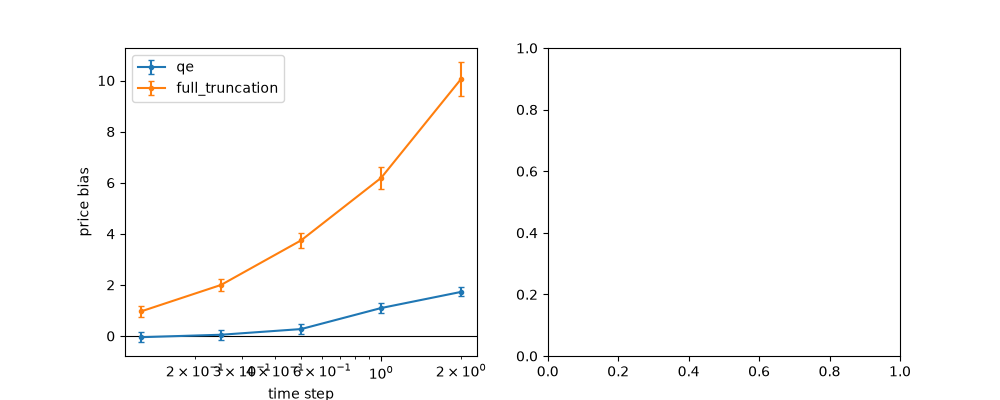
Leif Andersen (2008) simulated the Heston variance by matching the mean and variance of its exact noncentral chi-square transition with something cheap to sample: a scaled squared Gaussian when the variance is well away from zero, and a point mass at zero plus an exponential tail when it is close, switching at \(\psi = s^2/m^2 = 1.5\). The spot then takes a step that integrates the variance with the trapezoidal rule. On Andersen’s hardest test case (Feller condition badly violated, ten years) QE is nearly unbiased with a few steps per year, where Euler schemes are far off.

import matplotlib.pyplot as plt
import numpy as np

from financialkit.stochastic_volatility import HestonModel, heston_mc_price, heston_paths

m = HestonModel(v0=0.04, kappa=0.5, theta=0.04, xi=1.0, rho=-0.9)
S, K, T, r = 100.0, 100.0, 10.0, 0.0
exact = m.price(S, K, T, r)
print(f"Andersen Case I, Feller satisfied: {m.feller_satisfied}; exact price {exact:.4f} (Andersen: 13.0847)")

Andersen Case I, Feller satisfied: False; exact price 13.0847 (Andersen: 13.0847)

Bias against step size

steps = np.array([5, 10, 20, 40, 80])
fig, (ax1, ax2) = plt.subplots(1, 2, figsize=(10, 4))
for scheme in ("qe", "full_truncation"):
    res = [heston_mc_price(m, S, K, T, r, n_steps=n, n_paths=20_000, scheme=scheme, rng=1) for n in steps]
    bias = np.array([x.estimate - exact for x in res])
    se = np.array([x.std_error for x in res])
    ax1.errorbar(T / steps, bias, yerr=2 * se, marker="o", ms=3, capsize=2, label=scheme)
ax1.axhline(0.0, color="k", lw=0.8)
ax1.set_xscale("log")
ax1.set_xlabel("time step")
ax1.set_ylabel("price bias")
ax1.legend()

<matplotlib.legend.Legend object at 0x117db0d70>

The variance hits zero

The exponential branch puts an atom at zero, as the exact transition has when the Feller condition fails.

v = heston_paths(m, S, 1.0, r, n_steps=10, n_paths=50_000, scheme="qe", rng=2).variance[:, -1]
print(f"fraction of paths with v(1) = 0: {np.mean(v == 0):.3f}")
ax2.hist(v[v > 0], bins=80, range=(0, 0.2))
ax2.set_xlabel("v(1)")
ax2.set_ylabel("paths")
ax2.set_title(f"QE variance after one year ({np.mean(v == 0):.0%} of paths at 0)")
fig.tight_layout()

plt.show()

fraction of paths with v(1) = 0: 0.793