Hagan’s SABR model

Hagan, Kumar, Lesniewski and Woodward (2002) observed that local volatility predicts the wrong dynamics: when the forward rises, a local volatility model moves the smile the wrong way. Their stochastic \(\alpha\beta\rho\) model, \(dF = \alpha F^\beta\,dW_1\), \(d\alpha = \nu\alpha\,dW_2\), has an asymptotic implied-volatility formula that became the market standard for swaption smiles. Each parameter has one job: \(\beta\) the backbone, \(\rho\) the skew, \(\nu\) the curvature. Here a smile is calibrated and each parameter varied in turn.

import matplotlib.pyplot as plt
import numpy as np

from financialkit.stochastic_volatility import sabr_calibrate, sabr_implied_vol
from financialkit.stochastic_volatility.visualizers import plot_smile

F, T = 0.03, 5.0
K = np.linspace(0.01, 0.06, 26)
alpha, beta = 0.035, 0.5  # at-the-money Black vol alpha / F^(1 - beta), about 20%

Calibration to a noisy smile

rng = np.random.default_rng(0)
market = sabr_implied_vol(F, K, T, alpha, beta, -0.3, 0.4) + rng.normal(0, 5e-4, K.size)
fit = sabr_calibrate(F, K, T, market, beta=beta)
print(f"true alpha = {alpha}, rho = -0.3, nu = 0.4")
print(f"fit  alpha = {fit.alpha:.4f}, rho = {fit.rho:.3f}, nu = {fit.nu:.3f}, rms error = {fit.rmse * 1e4:.1f} bp of vol")

fig, axes = plt.subplots(1, 3, figsize=(12, 3.8))
axes[0].plot(K, market, "o", ms=3, label="market")
plot_smile(K, fit.implied_vol(K), ax=axes[0], label="SABR fit")

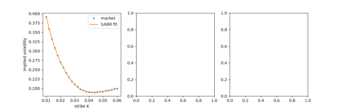
true alpha = 0.035, rho = -0.3, nu = 0.4
fit  alpha = 0.0349, rho = -0.299, nu = 0.402, rms error = 3.8 bp of vol

<Axes: xlabel='strike K', ylabel='implied volatility'>

Correlation and vol of vol

for rho in (-0.6, 0.0, 0.6):
    plot_smile(K, sabr_implied_vol(F, K, T, alpha, beta, rho, 0.4), ax=axes[1], label=f"rho = {rho}")
for nu in (0.1, 0.4, 0.8):
    plot_smile(K, sabr_implied_vol(F, K, T, alpha, beta, 0.0, nu), ax=axes[2], label=f"nu = {nu}")
fig.tight_layout()

plt.show()