Lee’s moment formula

Roger Lee (2004) proved that the total implied variance can grow at most linearly in the log strike, and that the slope is fixed by how many moments the price has. If \(\tilde p\) is the supremum of the \(p\) with \(E[S_T^{1+p}] < \infty\), then

\[\limsup_{k \to \infty} \frac{\sigma_{BS}^2(k)\,T}{k} = 2 - 4\left(\sqrt{\tilde p^2 + \tilde p} - \tilde p\right),\]

and the left wing obeys the same formula with the negative moments. Kou’s model makes this concrete: its exponential jump tails give \(\tilde p = \eta_1 - 1\) and \(\tilde q = \eta_2\). The bound is approached slowly, with corrections of order \(\ln|k|/|k|\).

import matplotlib.pyplot as plt
import numpy as np

from financialkit.stochastic_volatility import KouModel, VarianceGammaModel, lee_wing_slope

S, r, T = 100.0, 0.0, 1.0
k = np.linspace(0.25, 6.0, 24)

fig, (ax1, ax2) = plt.subplots(1, 2, figsize=(10, 4))
for eta1, eta2 in ((3.0, 2.0), (6.0, 4.0)):
    m = KouModel(0.1, 1.0, 0.5, eta1, eta2)
    p, q = m.critical_moments()
    right = m.implied_vol(S, S * np.exp(k), T, r) ** 2 * T / k
    left = m.implied_vol(S, S * np.exp(-k), T, r) ** 2 * T / k
    line = ax1.plot(k, right, label=f"right wing, eta1 = {eta1:g}")[0]
    ax1.axhline(lee_wing_slope(p), color=line.get_color(), ls="--", lw=1)
    line = ax2.plot(k, left, label=f"left wing, eta2 = {eta2:g}")[0]
    ax2.axhline(lee_wing_slope(q), color=line.get_color(), ls="--", lw=1)
    print(f"eta1 = {eta1:g}, eta2 = {eta2:g}: critical moments p = {p:g}, q = {q:g}; Lee slopes {lee_wing_slope(p):.4f}, {lee_wing_slope(q):.4f}")
for ax in (ax1, ax2):
    ax.set_xlabel("|log-moneyness| |k|")
    ax.set_ylabel("w(k) / |k|")
    ax.set_ylim(0, 1)
    ax.legend()
ax1.set_title("dashed: Lee's bound")
fig.tight_layout()

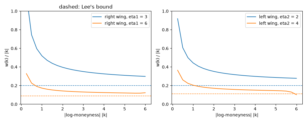
eta1 = 3, eta2 = 2: critical moments p = 2, q = 2; Lee slopes 0.2020, 0.2020
eta1 = 6, eta2 = 4: critical moments p = 5, q = 4; Lee slopes 0.0911, 0.1115

Variance gamma

p, q = VarianceGammaModel(0.2, 0.5, -0.2).critical_moments()
print(f"variance gamma: p = {p:.3f}, q = {q:.3f}, wing slopes {lee_wing_slope(p):.4f} (right), {lee_wing_slope(q):.4f} (left)")

plt.show()

variance gamma: p = 15.180, q = 6.180, wing slopes 0.0319 (right), 0.0750 (left)