Box-Jenkins ARMA

George Box and Gwilym Jenkins (1970) turned the mixed autoregressive moving-average model

\[\phi(B)(x_t - \mu) = \theta(B)\,\varepsilon_t\]

into a three-stage method. Identify the orders from the autocorrelation function (which cuts off after lag \(q\) for a pure MA) and the partial autocorrelation function (which cuts off after lag \(p\) for a pure AR); estimate by maximum likelihood; check that the residuals are white noise; then forecast. Here the cycle is run on a simulated ARMA(1,1), such as a spread or a monthly growth rate might follow.

import matplotlib.pyplot as plt
import numpy as np

from financialkit.time_series import fit_arma, ljung_box, simulate_arma
from financialkit.time_series.visualizers import plot_acf

x = simulate_arma(ar=[0.75], ma=[0.4], n=600, mean=2.0, rng=3)

Identification

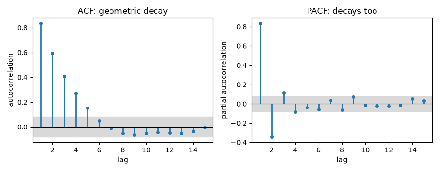
Neither function cuts off: both decay, which points to a mixed model.

fig, (ax1, ax2) = plt.subplots(1, 2, figsize=(9, 3.5))
plot_acf(x, 15, ax=ax1)
plot_acf(x, 15, partial=True, ax=ax2)
ax1.set_title("ACF: geometric decay")
ax2.set_title("PACF: decays too")
fig.tight_layout()

Estimation and diagnostic checking

Conditional maximum likelihood recovers \(\phi = 0.75\) and \(\theta = 0.4\), and the Ljung-Box test finds no correlation left in the residuals (two degrees of freedom are used up by the fit).

res = fit_arma(x, 1, 1)
lb = ljung_box(res.residuals, lags=12, fitted_params=2)
print(f"phi = {res.ar[0]:.3f}, theta = {res.ma[0]:.3f}, mu = {res.mean:.3f}, sigma^2 = {res.sigma2:.3f}")
print(f"Ljung-Box on residuals: Q = {lb.statistic:.1f}, p = {lb.pvalue:.2f}")

phi = 0.724, theta = 0.447, mu = 2.110, sigma^2 = 0.990
Ljung-Box on residuals: Q = 11.8, p = 0.30

Forecasting

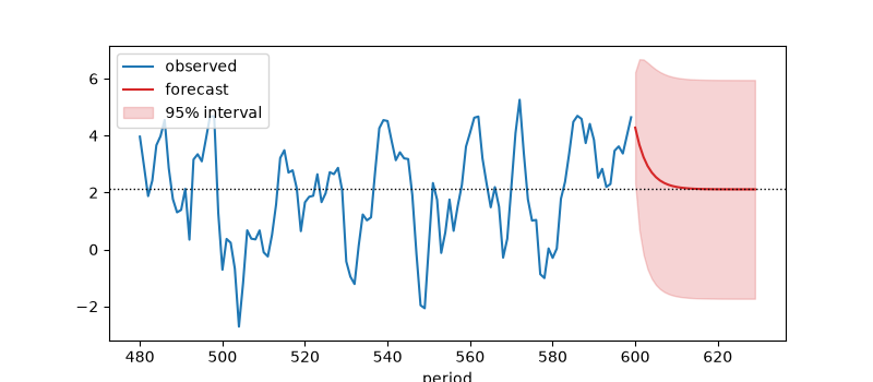
Forecasts decay geometrically back to the mean, and the 95% interval widens to the unconditional spread.

h = 30
mean, se = res.forecast(h)
t = np.arange(x.size)
tf = np.arange(x.size, x.size + h)
fig, ax = plt.subplots(figsize=(8, 3.5))
ax.plot(t[-120:], x[-120:], color="C0", label="observed")
ax.plot(tf, mean, color="C3", label="forecast")
ax.fill_between(tf, mean - 1.96 * se, mean + 1.96 * se, color="C3", alpha=0.2, label="95% interval")
ax.axhline(res.mean, color="k", ls=":", lw=1)
ax.set_xlabel("period")
ax.legend(loc="upper left")
plt.show()