Hill tail index

If the tail is a power law, \(P(X > u) \approx C u^{-\alpha}\), the log-excesses of the largest observations over a threshold are exponential with mean \(1/\alpha\). Bruce Hill (1975) turned this into the estimator

\[\hat\alpha_k = \Bigl[\frac1k\sum_{i=1}^{k}\ln X_{(i)} - \ln X_{(k+1)}\Bigr]^{-1},\]

using only the \(k\) largest order statistics. The tail index decides which moments exist (those of order below \(\alpha\)), and so whether the variance and kurtosis that risk models rely on are finite.

import matplotlib.pyplot as plt
import numpy as np

from financialkit.time_series import EGARCH, hill_estimator
from financialkit.time_series.visualizers import plot_hill

The Hill plot

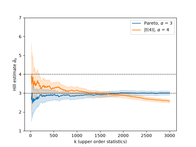
For an exact Pareto tail the estimate is flat in \(k\). For a Student t with \(\nu = 4\), only the far tail is a power law, so the estimate drifts once \(k\) reaches into the body: choosing \(k\) trades variance (small \(k\)) against bias (large \(k\)).

rng = np.random.default_rng(1975)
n = 20_000
pareto = rng.pareto(3.0, n) + 1.0
student = np.abs(rng.standard_t(4, n))

fig, ax = plt.subplots()
plot_hill(hill_estimator(pareto, k=np.arange(20, 3000)), ax=ax, label=r"Pareto, $\alpha$ = 3")
plot_hill(hill_estimator(student, k=np.arange(20, 3000)), ax=ax, label=r"|t(4)|, $\alpha$ = 4")
for a in (3, 4):
    ax.axhline(a, color="k", ls="--", lw=0.8)
ax.set_ylim(1, 7)

(1.0, 7.0)

Fat tails from volatility clustering

Returns with Gaussian innovations but a changing variance also have power-law tails. The left and right tails of an EGARCH model with a leverage effect differ: the left one is fatter.

r = EGARCH(omega=0.0, alpha=0.25, gamma=-0.12, beta=0.97).simulate(n, rng=1).returns
k = np.arange(50, 1500)
fig, ax = plt.subplots()
plot_hill(hill_estimator(r, k=k, side="lower"), ax=ax, label="losses (left tail)")
plot_hill(hill_estimator(r, k=k, side="upper"), ax=ax, label="gains (right tail)")
ax.set_title("EGARCH returns with normal innovations")
for side in ("lower", "upper"):
    print(f"{side} tail: alpha at k = 500 is {hill_estimator(r, k=500, side=side).alpha[0]:.2f}")
plt.show()

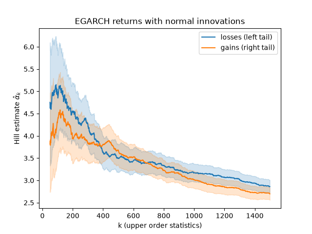
lower tail: alpha at k = 500 is 3.50
upper tail: alpha at k = 500 is 3.68