Dickey-Fuller unit roots

Is a series a random walk (\(\rho = 1\)) or does it revert to a mean (\(\rho < 1\))? Regressing \(\Delta y_t\) on \(y_{t-1}\) and looking at the t-ratio of the slope seems natural, but under a unit root that ratio does not have a t distribution: it is skewed to the left, and more so when a constant or trend is included. David Dickey and Wayne Fuller (1979) tabulated its distribution by simulation. Their test, with lagged differences added (Said and Dickey 1984) and MacKinnon’s critical values, is still the first thing run on an interest rate, a price-dividend ratio or a pairs-trading spread.

import matplotlib.pyplot as plt
import numpy as np
from scipy import stats

from financialkit.time_series import adf_test, mackinnon_critical_values, simulate_arma
from financialkit.time_series.utils import simulate_dickey_fuller

The Dickey-Fuller distributions

Ten thousand random walks of length 250, tested with no deterministic terms, a constant, and a constant and trend. The 5% critical values (vertical lines) lie far to the left of the normal’s \(-1.645\).

T = 250
fig, ax = plt.subplots()
g = np.linspace(-5, 3, 300)
ax.plot(g, stats.norm.pdf(g), "k", lw=1, label="N(0, 1)")
for i, (reg, label) in enumerate((("n", "none"), ("c", "constant"), ("ct", "constant + trend"))):
    tau = simulate_dickey_fuller(T, 10_000, reg, rng=i)
    ax.hist(tau, bins=60, density=True, histtype="step", lw=1.5, color=f"C{i}", label=label)
    cv = mackinnon_critical_values(T, reg)["5%"]
    ax.axvline(cv, color=f"C{i}", ls="--", lw=1)
    print(f"{label:16s} simulated 5% quantile {np.quantile(tau, 0.05):.3f}, MacKinnon {cv:.3f}")
ax.set_xlabel("t-ratio of gamma")
ax.legend()

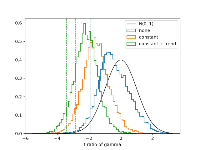
none             simulated 5% quantile -1.924, MacKinnon -1.942
constant         simulated 5% quantile -2.861, MacKinnon -2.873
constant + trend simulated 5% quantile -3.457, MacKinnon -3.428

<matplotlib.legend.Legend object at 0x116d7cc20>

Testing two rates

A short rate that mean-reverts (\(\rho = 0.95\) a month) and one that is a random walk look alike over 30 years. The augmented test rejects a unit root for the first and not for the second. At this sample size it detects \(\rho = 0.95\) only about four times in five, and its power falls fast as \(\rho \to 1\), so failing to reject is weak evidence of a unit root.

rng = np.random.default_rng(0)
months = 360
reverting = 0.04 + simulate_arma(ar=[0.95], n=months, sigma=0.002, rng=rng)
walk = 0.04 + np.cumsum(0.002 * rng.standard_normal(months))
fig, ax = plt.subplots(figsize=(8, 3))
for name, x in (("mean-reverting", reverting), ("random walk", walk)):
    res = adf_test(x, regression="c")
    ax.plot(100 * x, label=f"{name}: ADF = {res.statistic:.2f}")
    print(f"{name:15s} ADF = {res.statistic:.2f} (5% cv {res.critical_values['5%']:.2f}), lags {res.lags}, reject: {res.rejects()}")
ax.set_xlabel("month")
ax.set_ylabel("rate (%)")
ax.legend()
plt.show()

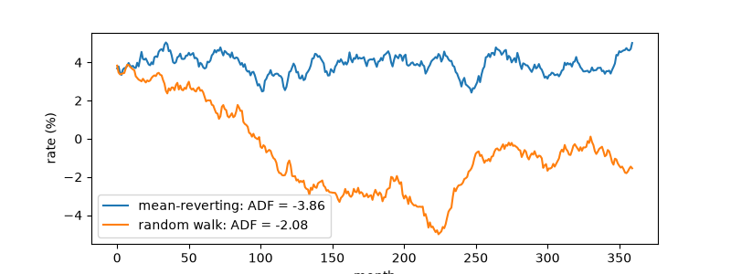
mean-reverting  ADF = -3.86 (5% cv -2.87), lags 3, reject: True
random walk     ADF = -2.08 (5% cv -2.87), lags 0, reject: False