Engle-Granger cointegration

Granger and Newbold (1974) showed that regressing one random walk on an independent one gives “significant” slopes and high \(R^2\) most of the time: a spurious regression. Yet some nonstationary series are tied together, such as spot and futures prices, or two share classes of the same company. Robert Engle and Clive Granger (1987) called them cointegrated: some combination \(y_t - b x_t\) is stationary. Their two-step test regresses \(y\) on \(x\) and runs a Dickey-Fuller test on the residuals, with critical values that allow for \(b\) having been fitted. It is the textbook basis of pairs trading.

import matplotlib.pyplot as plt
import numpy as np

from financialkit.time_series import engle_granger
from financialkit.time_series.utils import simulate_cointegrated_pair

A cointegrated pair and a spurious one

Two log prices that share a stochastic trend (the spread is an AR(1) with a half-life of about a week), and two independent random walks.

rng = np.random.default_rng(1987)
n = 750
y, x = simulate_cointegrated_pair(n, beta=1.2, intercept=0.5, phi=0.9, sigma_x=0.02, sigma_u=0.01, rng=rng)
a, b = np.cumsum(0.02 * rng.standard_normal(n)), np.cumsum(0.02 * rng.standard_normal(n))

coint = engle_granger(y, x)
spur = engle_granger(a, b)
for name, res in (("cointegrated", coint), ("spurious", spur)):
    cv = res.critical_values["5%"]
    print(f"{name:13s} b = {res.beta[0]:6.3f}, R^2 = {res.r_squared:.2f}, EG = {res.statistic:6.2f} (5% cv {cv:.2f}), reject: {res.rejects()}")

fig, axes = plt.subplots(2, 2, figsize=(9, 5.5), sharex=True)
axes[0, 0].plot(y, label="y")
axes[0, 0].plot(x, label="x")
axes[0, 0].set_title("cointegrated pair")
axes[0, 0].legend()
axes[1, 0].plot(coint.residuals, color="C2")
axes[1, 0].set_title("spread $y - a - bx$: stationary")
axes[0, 1].plot(a)
axes[0, 1].plot(b)
axes[0, 1].set_title(f"independent walks, $R^2$ = {spur.r_squared:.2f}")
axes[1, 1].plot(spur.residuals, color="C3")
axes[1, 1].set_title("residual: still a random walk")
for ax in axes[1]:
    ax.set_xlabel("day")
fig.tight_layout()

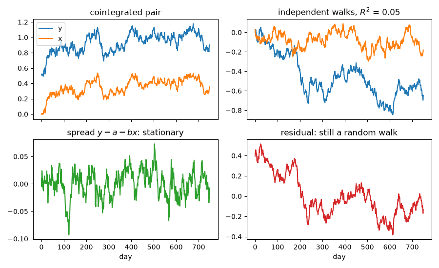
cointegrated  b =  1.195, R^2 = 0.96, EG =  -6.01 (5% cv -3.34), reject: True
spurious      b =  0.592, R^2 = 0.05, EG =  -2.13 (5% cv -3.34), reject: False

Spurious regression in numbers

Across 300 pairs of independent walks the slope’s naive t-ratio exceeds 2 in most of them, but the Engle-Granger test rejects close to its 5% size.

big_t, eg_reject = [], []
for _ in range(300):
    a, b = np.cumsum(rng.standard_normal((2, 250)), axis=1)
    X = np.column_stack([np.ones(250), b])
    coef, res, *_ = np.linalg.lstsq(X, a, rcond=None)
    se = np.sqrt(res[0] / 248 * np.linalg.inv(X.T @ X)[1, 1])
    big_t.append(abs(coef[1] / se) > 2)
    eg_reject.append(engle_granger(a, b, lags=0).rejects())
print(f"|t| > 2 in {np.mean(big_t):.0%} of spurious regressions; Engle-Granger rejects in {np.mean(eg_reject):.0%}")
plt.show()

|t| > 2 in 84% of spurious regressions; Engle-Granger rejects in 3%