Jensen’s alpha

Michael Jensen (1968) measured a mutual fund’s skill as the intercept of its excess return regressed on the market’s,

\[r_{pt} - r_{ft} = \alpha_p + \beta_p (r_{mt} - r_{ft}) + \varepsilon_{pt}.\]

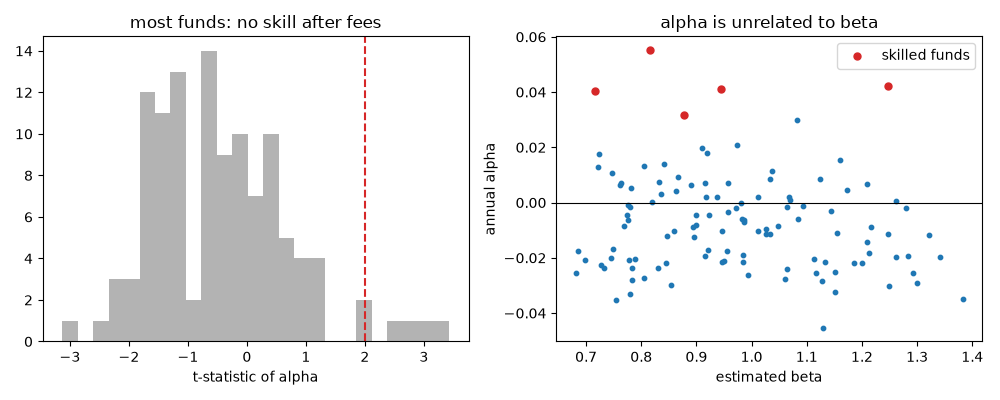
A manager who takes more market risk earns more on average but no alpha; only returns beyond the security market line count. Over 1945-1964 Jensen found the average alpha of 115 funds to be negative after fees, and no more funds with significant positive alpha than chance allows.

import matplotlib.pyplot as plt
import numpy as np

from financialkit.asset_pricing import jensen_alpha, simulate_factor_model

rng = np.random.default_rng(1968)
n_funds, T = 115, 240
betas = rng.uniform(0.7, 1.3, n_funds)
# Fees of 1% a year and no skill, except five genuinely skilled funds.
true_alpha = np.full(n_funds, -0.01 / 12)
true_alpha[:5] = 0.04 / 12
panel = simulate_factor_model(T, betas, [0.006], [[0.0020]], idio_vol=0.02, alphas=true_alpha, rng=rng)
res = jensen_alpha(panel.excess_returns, panel.factors[:, 0])
print(f"mean annual alpha: {12 * res.alphas.mean():+.2%}")
print(f"funds with alpha t > 2: {(res.alpha_t > 2).sum()} (true skilled: 5)")

mean annual alpha: -0.70%
funds with alpha t > 2: 4 (true skilled: 5)

fig, axes = plt.subplots(1, 2, figsize=(10, 4))
axes[0].hist(res.alpha_t, bins=25, color="0.7")
axes[0].axvline(2, color="C3", ls="--")
axes[0].set_xlabel("t-statistic of alpha")
axes[0].set_title("most funds: no skill after fees")
axes[1].scatter(res.betas[:, 0], 12 * res.alphas, s=10)
axes[1].scatter(res.betas[:5, 0], 12 * res.alphas[:5], s=25, color="C3", label="skilled funds")
axes[1].axhline(0, color="k", lw=0.8)
axes[1].set_xlabel("estimated beta")
axes[1].set_ylabel("annual alpha")
axes[1].set_title("alpha is unrelated to beta")
axes[1].legend()
fig.tight_layout()

plt.show()