The Gibbons-Ross-Shanken test

Testing the CAPM means asking whether the market portfolio is mean-variance efficient, that is whether the time-series alphas of a set of test assets are jointly zero. Michael Gibbons, Stephen Ross and Jay Shanken (1989) gave the exact finite-sample distribution under normal errors:

\[\frac{T - N - K}{N}\,\frac{\hat\alpha'\hat\Sigma^{-1}\hat\alpha}{1 + \bar f'\hat\Omega^{-1}\bar f} \sim F_{N,\,T-N-K}.\]

The statistic measures how far the tangency portfolio of factors and test assets together beats the factors alone in squared Sharpe ratio.

import matplotlib.pyplot as plt
import numpy as np
from scipy import stats

from financialkit.asset_pricing import grs_test, simulate_factor_model

rng = np.random.default_rng(1989)
T, N = 120, 10
betas = np.linspace(0.6, 1.4, N)

# Under the null the p-values are uniform: the test has the right size.
p_null = [grs_test(p.excess_returns, p.factors).p_value for p in (simulate_factor_model(T, betas, [0.006], [[0.002]], rng=rng) for _ in range(400))]
stat_null = [stats.f.isf(p, N, T - N - 1) for p in p_null]

fig, axes = plt.subplots(1, 2, figsize=(10, 4))
x = np.linspace(0, 4, 200)
axes[0].hist(stat_null, bins=30, density=True, color="0.75", label="simulated GRS under H0")
axes[0].plot(x, stats.f.pdf(x, N, T - N - 1), "C3", label=f"F({N}, {T - N - 1})")
axes[0].set_xlabel("GRS statistic")
axes[0].legend()
print(f"rejection rate at 5% under H0: {np.mean(np.array(p_null) < 0.05):.3f}")

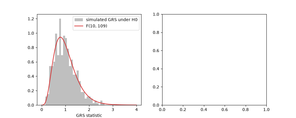
rejection rate at 5% under H0: 0.043

Power against mispricing

alphas = np.linspace(0, 0.006, 7)
power = []
for a in alphas:
    pa = [
        grs_test(p.excess_returns, p.factors).reject()
        for p in (simulate_factor_model(T, betas, [0.006], [[0.002]], alphas=a * np.linspace(-1, 1, N), rng=rng) for _ in range(100))
    ]
    power.append(np.mean(pa))
axes[1].plot(12 * alphas, power, "o-")
axes[1].set_xlabel("largest |alpha| per year")
axes[1].set_ylabel("rejection rate")
axes[1].set_title(f"T = {T} months, N = {N} assets")
fig.tight_layout()

plt.show()