Black’s zero-beta CAPM

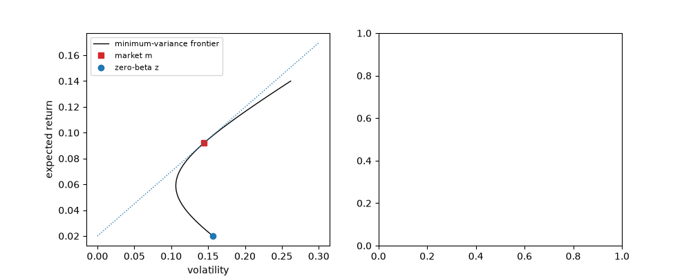
Sharpe’s CAPM assumes unlimited riskless borrowing. Fischer Black (1972) dropped it: every frontier portfolio \(m\) still prices all assets linearly, with the expected return of \(z\), the minimum-variance portfolio uncorrelated with \(m\), in place of the riskless rate,

\[E[r_i] = E[r_z] + \beta_{im} (E[r_m] - E[r_z]).\]

Since \(E[r_z]\) lies above the lending rate, the security market line is flatter than Sharpe’s, which matched Black, Jensen and Scholes’s (1972) finding that low-beta stocks earn more, and high-beta ones less, than the CAPM predicts.

import matplotlib.pyplot as plt
import numpy as np

from financialkit.asset_pricing import zero_beta_capm

mu = np.array([0.05, 0.07, 0.09, 0.11, 0.13])
vol = np.array([0.12, 0.16, 0.20, 0.25, 0.32])
cov = (0.3 + 0.7 * np.eye(5)) * np.outer(vol, vol)
res = zero_beta_capm(mu, cov, zero_beta_rate=0.02)
wz, wm = res.zero_beta_weights, res.market_weights
print(f"E[r_z] = {res.zero_beta_rate:.4f},  cov(z, m) = {wz @ cov @ wm:.2e}")

E[r_z] = 0.0200,  cov(z, m) = 1.52e-18

The frontier, the market and its zero-beta portfolio

ones = np.ones(5)
Ci = np.linalg.inv(cov)
A, B, C = ones @ Ci @ mu, mu @ Ci @ mu, ones @ Ci @ ones
targets = np.linspace(0.02, 0.14, 200)
sd = np.sqrt((C * targets**2 - 2 * A * targets + B) / (B * C - A**2))
fig, axes = plt.subplots(1, 2, figsize=(10, 4))
axes[0].plot(sd, targets, "k", lw=1, label="minimum-variance frontier")
axes[0].plot(np.sqrt(wm @ cov @ wm), res.market_return, "s", color="C3", label="market m")
axes[0].plot(np.sqrt(wz @ cov @ wz), res.zero_beta_rate, "o", color="C0", label="zero-beta z")
x = np.linspace(0, 0.3, 2)
axes[0].plot(x, res.zero_beta_rate + (res.market_return - res.zero_beta_rate) / np.sqrt(wm @ cov @ wm) * x, "C0", ls=":", lw=1)
axes[0].set_xlabel("volatility")
axes[0].set_ylabel("expected return")
axes[0].legend(fontsize=8)

<matplotlib.legend.Legend object at 0x116ab46e0>

The security market line starts at E[r_z]

b = np.linspace(0, 1.6, 2)
axes[1].plot(res.betas, mu, "o", color="C1", label="assets")
axes[1].plot(b, res.zero_beta_rate + b * (res.market_return - res.zero_beta_rate), "C0", label="zero-beta SML")
rf = 0.005
axes[1].plot(b, rf + b * (res.market_return - rf), "C3", ls="--", label=f"Sharpe SML with r_f = {rf:.1%}")
axes[1].set_xlabel("beta on m")
axes[1].legend(fontsize=8)
fig.tight_layout()

plt.show()