Lucas’s tree

Robert Lucas (1978) priced assets in the simplest economy that has them: a representative agent with power utility owns a tree whose fruit is the only consumption good. Prices must make the agent content to hold the tree and eat its dividend, which gives the Euler equation

\[P_t = E_t\left[\beta \left(\frac{C_{t+1}}{C_t}\right)^{-\gamma} (P_{t+1} + D_{t+1})\right], \qquad C = D.\]

With i.i.d. lognormal growth the price-dividend ratio is constant, so the price inherits the dividend’s random walk. The riskless rate and the equity premium follow from just \(\beta\), \(\gamma\) and the mean and volatility of consumption growth.

import matplotlib.pyplot as plt
import numpy as np

from financialkit.asset_pricing import LucasTree

tree = LucasTree(beta=0.97, gamma=2.0, mu=0.02, sigma=0.036)
m = tree.moments()
print(f"P/D = {m.price_dividend:.1f},  R_f = {m.risk_free - 1:.2%},  E[R_e] = {m.equity_return - 1:.2%},  premium = {m.equity_premium:.2%}")

path = tree.simulate(100, rng=1978)
D = np.cumprod(np.concatenate([[1.0], path.growth]))
fig, ax = plt.subplots(figsize=(8, 3.5))
ax.semilogy(D * m.price_dividend, label="price P_t")
ax.semilogy(D, "C3", lw=1, label="dividend D_t")
ax.set_xlabel("year")
ax.set_ylabel("price")
ax.set_title("the price is a constant multiple of the dividend")
ax.legend()
fig.tight_layout()

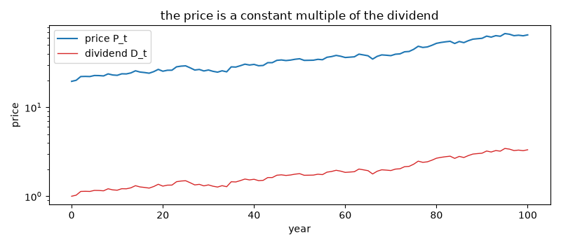
P/D = 19.6,  R_f = 7.02%,  E[R_e] = 7.30%,  premium = 0.28%

Prices and returns across risk aversion

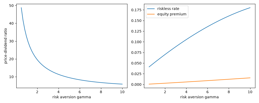
Higher \(\gamma\) raises the riskless rate (the agent wants to borrow against future growth) but adds only \(\gamma\sigma^2\) to the log premium.

gammas = np.linspace(0.5, 10, 60)
ms = [LucasTree(0.97, g, 0.02, 0.036).moments() for g in gammas]
fig, axes = plt.subplots(1, 2, figsize=(10, 4))
axes[0].plot(gammas, [x.price_dividend for x in ms])
axes[0].set_xlabel("risk aversion gamma")
axes[0].set_ylabel("price-dividend ratio")
axes[1].plot(gammas, [x.risk_free - 1 for x in ms], label="riskless rate")
axes[1].plot(gammas, [x.equity_premium for x in ms], label="equity premium")
axes[1].set_xlabel("risk aversion gamma")
axes[1].legend()
fig.tight_layout()

plt.show()