Breeden’s consumption CAPM

Merton’s intertemporal CAPM needs a beta for every state variable that shifts investment opportunities. Douglas Breeden (1979) showed that they all collapse into one: since optimal consumption already responds to every state variable, an asset’s risk premium is proportional to its covariance with aggregate consumption growth,

\[E[R_i] - R_f \approx \gamma\,\mathrm{Cov}(R_i, \Delta c) = \gamma\,\beta_{i,c}\,\sigma_c^2.\]

Assets that pay off when consumption is low are insurance and earn less.

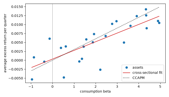
price of consumption risk: 0.00242 (true gamma sigma_c^2 = 0.00300)
implied gamma: 24.2

import matplotlib.pyplot as plt
import numpy as np

from financialkit.asset_pricing import ccapm_expected_excess_return, estimate_beta

rng = np.random.default_rng(1979)
T, N, gamma, sigma_c = 400, 25, 30.0, 0.01  # quarterly data
dc = 0.005 + sigma_c * rng.standard_normal(T)
beta_c = np.linspace(-1.0, 5.0, N)
premia = ccapm_expected_excess_return(beta_c, sigma_c, gamma)
R = premia + np.outer(dc - dc.mean(), beta_c) + 0.06 * rng.standard_normal((T, N))

b_hat = estimate_beta(R, dc)
slope, intercept = np.polyfit(b_hat, R.mean(axis=0), 1)
print(f"price of consumption risk: {slope:.5f} (true gamma sigma_c^2 = {gamma * sigma_c**2:.5f})")
print(f"implied gamma: {slope / sigma_c**2:.1f}")

fig, ax = plt.subplots(figsize=(7, 4))
ax.plot(b_hat, R.mean(axis=0), "o", label="assets")
bb = np.linspace(b_hat.min(), b_hat.max(), 2)
ax.plot(bb, intercept + slope * bb, "C3", label="cross-sectional fit")
ax.plot(bb, ccapm_expected_excess_return(bb, sigma_c, gamma), "k:", label="CCAPM")
ax.axvline(0, color="0.6", lw=0.8)
ax.set_xlabel("consumption beta")
ax.set_ylabel("average excess return per quarter")
ax.legend()
fig.tight_layout()

plt.show()