The equity premium puzzle

Rajnish Mehra and Edward Prescott (1985) calibrated a two-state version of Lucas’s economy to US consumption growth from 1889 to 1978 (mean 1.8%, standard deviation 3.6%, autocorrelation -0.14). Over the same period stocks earned 6.98% a year and short-term bills 0.80%: a premium of 6.18%. Searching over every time preference \(\beta < 1\) and risk aversion \(\gamma \le 10\), they could produce a premium of at most 0.35% while keeping the riskless rate below 4%. Consumption is simply too smooth for stocks to be that risky to a power-utility agent.

import matplotlib.pyplot as plt
import numpy as np

from financialkit.asset_pricing import MehraPrescott, implied_risk_aversion

points = []
for g in np.linspace(0.1, 10, 40):
    for b in np.linspace(0.85, 0.9999, 40):
        try:
            m = MehraPrescott(b, g).moments()
        except ValueError:
            continue
        points.append((m.risk_free - 1, m.equity_premium))
pts = np.array(points)
ok = (pts[:, 0] >= 0) & (pts[:, 0] <= 0.04)
print(f"largest premium with 0 <= r_f <= 4%: {pts[ok, 1].max():.2%}")

fig, ax = plt.subplots(figsize=(7, 4.5))
ax.scatter(100 * pts[:, 0], 100 * pts[:, 1], s=4, c="0.6", label="model, gamma <= 10, beta < 1")
ax.scatter(100 * pts[ok, 0], 100 * pts[ok, 1], s=4, c="C0", label="... with 0 <= r_f <= 4%")
ax.plot(0.80, 6.18, "*", color="C3", ms=14, label="US data 1889-1978")
ax.set_xlim(-2, 20)
ax.set_xlabel("average riskless rate (%)")
ax.set_ylabel("equity premium (%)")
ax.legend()
fig.tight_layout()

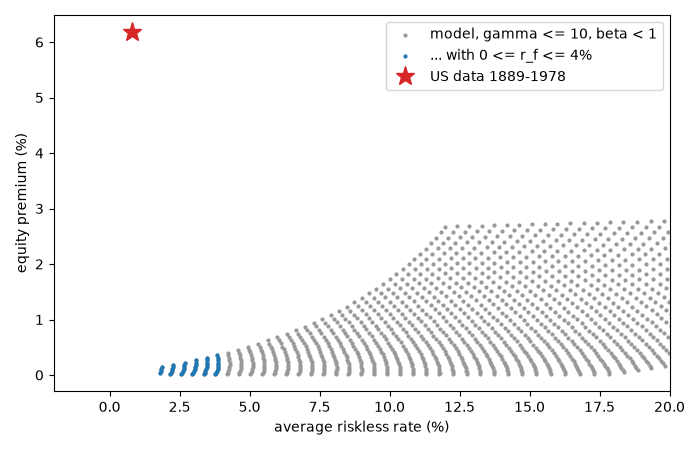
largest premium with 0 <= r_f <= 4%: 0.35%

How much risk aversion would it take?

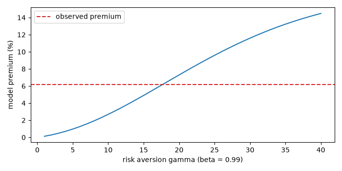
With the observed 16.5% equity volatility and 3.6% consumption volatility, the consumption CAPM needs \(\gamma\) above 10 even if stocks and consumption were perfectly correlated; with a realistic correlation of about 0.4 it needs about 26.

for rho in (1.0, 0.4):
    print(f"correlation {rho}: gamma = {implied_risk_aversion(0.0618, 0.1654, 0.036, rho):.0f}")

gammas = np.linspace(1, 40, 40)
prem = [MehraPrescott(0.99, g).moments().equity_premium for g in gammas]
fig, ax = plt.subplots(figsize=(7, 3.5))
ax.plot(gammas, 100 * np.array(prem))
ax.axhline(6.18, color="C3", ls="--", label="observed premium")
ax.set_xlabel("risk aversion gamma (beta = 0.99)")
ax.set_ylabel("model premium (%)")
ax.legend()
fig.tight_layout()

plt.show()

correlation 1.0: gamma = 10
correlation 0.4: gamma = 26