Williams’s dividend discount model

John Burr Williams (1938) defined the investment value of a stock as the present value of all the dividends it will ever pay,

\[V_0 = \sum_{t=1}^{\infty} \frac{D_t}{(1 + r)^t}.\]

Earnings matter only through the dividends they eventually fund. In practice an analyst forecasts a few years of dividends explicitly and then assumes steady growth, so most of the value often sits in the terminal value beyond the forecast horizon.

import matplotlib.pyplot as plt
import numpy as np

from financialkit.asset_pricing import dividend_discount_value

r = 0.09
# Five years of fast growth from a dividend of 1, then 3% forever.
divs = 1.0 * 1.12 ** np.arange(1, 6)
value = dividend_discount_value(divs, r, terminal_growth=0.03)
explicit = dividend_discount_value(divs, r)
print(f"value = {value:.2f}, of which explicit dividends {explicit:.2f} ({explicit / value:.0%})")

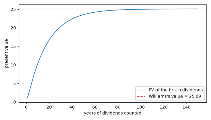
value = 25.09, of which explicit dividends 5.43 (22%)

Where the value comes from

Truncating the sum after \(n\) years shows how slowly the present value of the dividends accumulates: decades of dividends are needed to reach the full value.

years = np.arange(1, 151)
path = np.concatenate([divs, divs[-1] * 1.03 ** np.arange(1, years.size - divs.size + 1)])
partial = np.array([dividend_discount_value(path[:n], r) for n in years])
fig, ax = plt.subplots(figsize=(7, 4))
ax.plot(years, partial, label="PV of the first n dividends")
ax.axhline(value, color="C3", ls="--", label=f"Williams's value = {value:.2f}")
ax.set_xlabel("years of dividends counted")
ax.set_ylabel("present value")
ax.legend()
fig.tight_layout()

Sensitivity to the discount rate

rates = np.linspace(0.06, 0.14, 50)
fig, ax = plt.subplots(figsize=(7, 3.5))
ax.plot(rates, [dividend_discount_value(divs, k, terminal_growth=0.03) for k in rates])
ax.set_xlabel("required return r")
ax.set_ylabel("value")
fig.tight_layout()

plt.show()