Shiller’s excess volatility

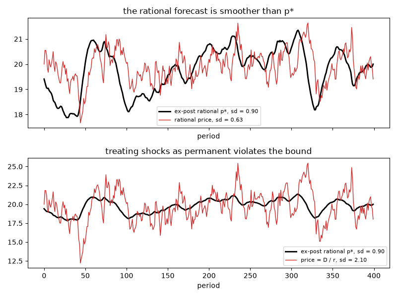
If a price is the rational forecast of discounted future dividends, \(p_t = E_t[p^*_t]\), then the ex-post rational price \(p^*_t\) computed from the dividends actually paid equals the price plus an unforecastable error. An optimal forecast varies less than the thing it forecasts, so \(\sigma(p) \le \sigma(p^*)\). Robert Shiller (1981) found US stock prices five to thirteen times too volatile for this bound.

Here dividends follow an AR(1) around a constant. The rational price respects the bound; a market that treats every dividend shock as permanent violates it.

import matplotlib.pyplot as plt
import numpy as np

from financialkit.asset_pricing import ar1_dividend_price, variance_bound
from financialkit.asset_pricing.visualizers import plot_excess_volatility

rng = np.random.default_rng(1981)
r, rho, Dbar, n = 0.05, 0.9, 1.0, 400
D = np.empty(n)
D[0] = Dbar
for t in range(1, n):
    D[t] = Dbar + rho * (D[t - 1] - Dbar) + 0.05 * rng.standard_normal()

rational = variance_bound(ar1_dividend_price(D, r, rho, Dbar), D, r, terminal_price=Dbar / r)
overreacting = variance_bound(D / r, D, r, terminal_price=Dbar / r)
print(f"rational price: sd ratio {rational.ratio:.2f}  (bound violated: {rational.violated})")
print(f"overreacting:   sd ratio {overreacting.ratio:.2f}  (bound violated: {overreacting.violated})")

rational price: sd ratio 0.70  (bound violated: False)
overreacting:   sd ratio 2.33  (bound violated: True)

fig, axes = plt.subplots(2, 1, figsize=(8, 6), sharex=True)
plot_excess_volatility(rational, ax=axes[0], label="rational price")
plot_excess_volatility(overreacting, ax=axes[1], label="price = D / r")
axes[0].set_title("the rational forecast is smoother than p*")
axes[1].set_title("treating shocks as permanent violates the bound")
fig.tight_layout()

plt.show()