Gordon growth

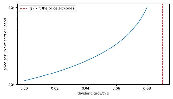
Myron Gordon (1959) summed Williams’s series for dividends that grow at a constant rate, \(P_0 = D_1 / (r - g)\), and connected the growth rate to the firm’s investment: a firm that retains a share \(b\) of its earnings and earns \(ROE\) on them grows at \(g = b \cdot ROE\). Read backwards, the model gives the market’s cost of equity as the dividend yield plus growth.

import matplotlib.pyplot as plt
import numpy as np

from financialkit.asset_pricing import gordon_growth_price, implied_cost_of_equity, sustainable_growth

r = 0.09
g = np.linspace(0.0, 0.08, 200)
fig, ax = plt.subplots(figsize=(7, 4))
ax.plot(g, gordon_growth_price(1.0, r, g))
ax.axvline(r, color="C3", ls="--", label="g -> r: the price explodes")
ax.set_xlabel("dividend growth g")
ax.set_ylabel("price per unit of next dividend")
ax.set_yscale("log")
ax.legend()
fig.tight_layout()

Growth from retained earnings

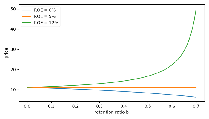
Retaining earnings adds value only if they earn more than the cost of equity. With earnings of 1 per share, \(D_1 = 1 - b\).

b = np.linspace(0.0, 0.7, 100)
fig, ax = plt.subplots(figsize=(7, 4))
for roe in (0.06, 0.09, 0.12):
    gb = sustainable_growth(roe, 1 - b)
    ax.plot(b, gordon_growth_price(1 - b, r, gb), label=f"ROE = {roe:.0%}")
ax.set_xlabel("retention ratio b")
ax.set_ylabel("price")
ax.legend()
fig.tight_layout()

The implied cost of equity

print(f"price 40, next dividend 2, growth 4%: r = {implied_cost_of_equity(40.0, 2.0, 0.04):.2%}")

plt.show()

price 40, next dividend 2, growth 4%: r = 9.00%