Merton’s structural model

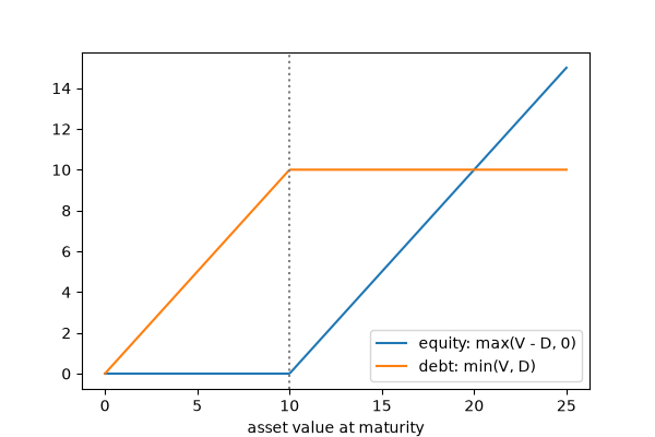
Merton (1974) treated a firm’s equity as a European call on its assets \(V\), struck at the face value \(D\) of its zero-coupon debt. Debt is then a riskless bond minus a put, the risk-neutral default probability is \(N(-d_2)\), and the credit spread follows from leverage and asset volatility alone. Hull’s Example 24.3 backs out the unobserved asset value and volatility from equity (3) and its volatility (80%).

import matplotlib.pyplot as plt
import numpy as np

from financialkit.credit import merton_calibrate, merton_model

m = merton_calibrate(E=3.0, sigma_E=0.80, D=10.0, T=1.0, r=0.05)
print(f"assets V = {m.asset_value:.2f}, sigma_V = {m.asset_volatility:.4f}")
print(f"debt = {m.debt:.2f}, PD = {m.default_probability:.1%}, spread = {1e4 * m.credit_spread:.0f} bp, recovery = {m.recovery_rate:.1%}")

assets V = 12.40, sigma_V = 0.2123
debt = 9.40, PD = 12.7%, spread = 124 bp, recovery = 90.3%

Payoffs at maturity

VT = np.linspace(0, 25, 300)
fig, ax = plt.subplots(figsize=(6, 4))
ax.plot(VT, np.maximum(VT - 10, 0), label="equity: max(V - D, 0)")
ax.plot(VT, np.minimum(VT, 10), label="debt: min(V, D)")
ax.axvline(10, color="0.5", ls=":")
ax.set_xlabel("asset value at maturity")
ax.legend()

<matplotlib.legend.Legend object at 0x116491a90>

The term structure of credit spreads

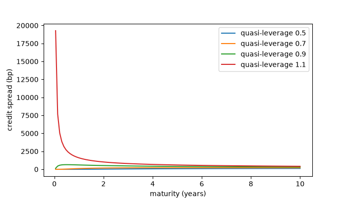
Merton’s spreads start at zero for very short maturities (assets cannot jump below the debt), rise, and for highly levered firms fall again because surviving firms drift away from default.

T = np.linspace(0.05, 10, 120)
fig, ax = plt.subplots(figsize=(7, 4))
for lev in (0.5, 0.7, 0.9, 1.1):
    s = [merton_model(100.0, 100 * lev * np.exp(0.05 * t), t, 0.05, 0.25).credit_spread for t in T]
    ax.plot(T, 1e4 * np.array(s), label=f"quasi-leverage {lev:.1f}")
ax.set_xlabel("maturity (years)")
ax.set_ylabel("credit spread (bp)")
ax.legend()

plt.show()