Crosbie and Bohn: the distance to default

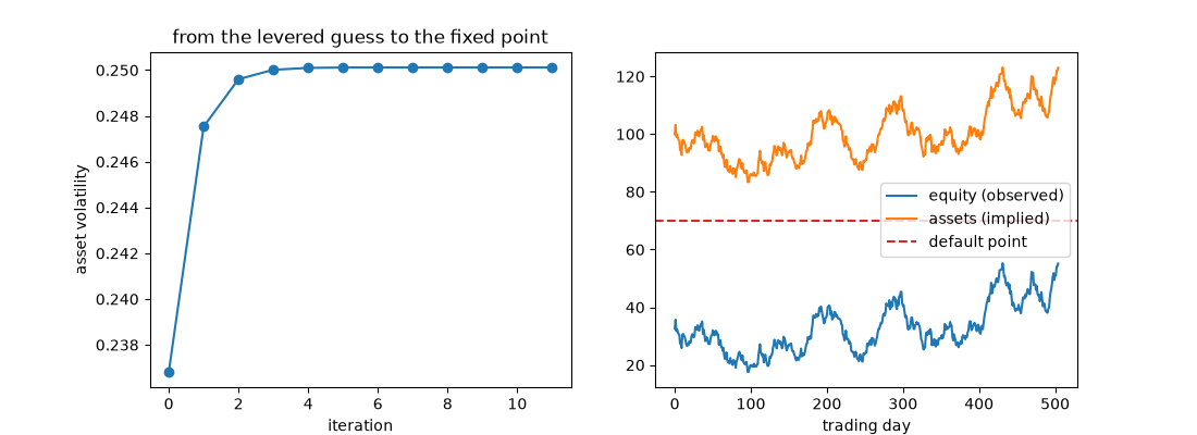
Moody’s KMV (Crosbie and Bohn 2003) turned Merton’s model into a default-prediction tool. Asset values are backed out from a daily equity series by iterating: guess the asset volatility, invert the equity call day by day, re-estimate the volatility from the implied asset returns, and repeat. The default point is short-term debt plus half the long-term debt, and the number of standard deviations between the assets and that point,

\[DD = \frac{\ln(V/D) + (\mu - \sigma_V^2/2)T}{\sigma_V\sqrt{T}},\]

ranks firms by default risk.

import matplotlib.pyplot as plt
import numpy as np

from financialkit.credit import kmv_default_point, kmv_iterate
from financialkit.integrators import gbm_paths
from financialkit.options import black_scholes_price

D = kmv_default_point(short_term_debt=40.0, long_term_debt=60.0)
_, V = gbm_paths(100.0, -0.10, 0.25, T=2.0, n_steps=504, n_paths=1, rng=3)
V = V[0]
E = np.asarray(black_scholes_price(V, D, 1.0, 0.03, 0.25))

res = kmv_iterate(E, D, r=0.03)
print(f"default point {D:.0f}; converged in {res.n_iter} iterations to sigma_V = {res.asset_volatility:.3f}")

default point 70; converged in 11 iterations to sigma_V = 0.250

The iteration

fig, ax = plt.subplots(1, 2, figsize=(11, 4))
ax[0].plot(res.volatility_history, "o-")
ax[0].set_xlabel("iteration")
ax[0].set_ylabel("asset volatility")
ax[0].set_title("from the levered guess to the fixed point")
days = np.arange(E.size)
ax[1].plot(days, E, label="equity (observed)")
ax[1].plot(days, res.asset_values, label="assets (implied)")
ax[1].axhline(D, color="C3", ls="--", label="default point")
ax[1].set_xlabel("trading day")
ax[1].legend()

<matplotlib.legend.Legend object at 0x1163b2cf0>

A rolling distance to default

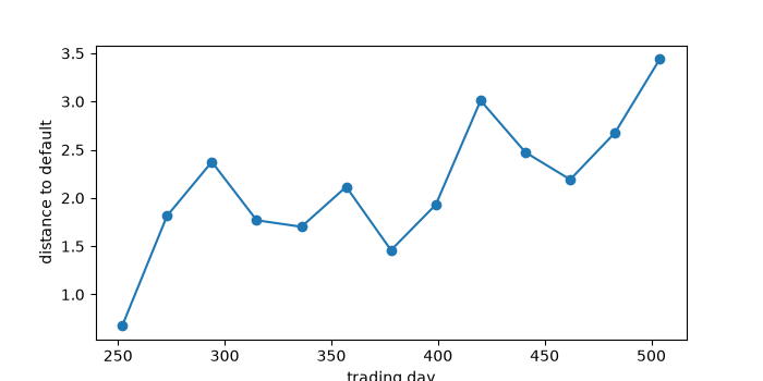
Re-running the estimate on a one-year window each month tracks how the firm drifts toward its default point.

ends = np.arange(252, E.size + 1, 21)
dd = [kmv_iterate(E[e - 252 : e], D, r=0.03).distance_to_default for e in ends]
fig, ax = plt.subplots(figsize=(7, 3.5))
ax.plot(ends, dd, "o-")
ax.set_xlabel("trading day")
ax.set_ylabel("distance to default")

plt.show()