The square-root impact law

A large order executed over a day moves the price by far less than proportionally to its size. Practitioners measured it in the 1980s and 1990s (Loeb, 1983; the BARRA market impact model of Torre, 1997): the impact of a metaorder of \(Q\) shares in a stock trading \(V\) shares a day with daily volatility \(\sigma\) is

\[I \approx Y\,\sigma\,\sqrt{Q / V},\]

with \(Y\) of order one, across markets, eras and asset classes. Doubling an order raises its cost per share by only 41%.

import matplotlib.pyplot as plt
import numpy as np

from financialkit.market_microstructure import fit_impact_law, square_root_impact

rng = np.random.default_rng(13)

Fitting the exponent to a set of metaorders

Synthetic metaorders follow the law with \(Y = 0.8\), plus multiplicative noise from everything else that moved the price.

n = 2000
participation = 10 ** rng.uniform(-4, -0.7, n)
sigma = rng.uniform(0.01, 0.03, n)
impact = square_root_impact(participation, 1.0, sigma, Y=0.8) * np.exp(0.5 * rng.standard_normal(n))
fit = fit_impact_law(participation, impact / sigma)
print(f"exponent {fit.coef[1]:.3f} ± {fit.std_errors[1]:.3f}, Y = {np.exp(fit.coef[0]):.2f}")

bins = np.logspace(-4, -0.7, 12)
idx = np.digitize(participation, bins)
centres = [np.exp(np.log(participation[idx == i]).mean()) for i in range(1, len(bins))]
means = [np.exp(np.log(impact[idx == i] / sigma[idx == i]).mean()) for i in range(1, len(bins))]
fig, ax = plt.subplots(figsize=(6, 4))
ax.loglog(participation, impact / sigma, ".", ms=2, color="0.75")
ax.loglog(centres, means, "o", color="C0", label="binned means")
q = np.logspace(-4, -0.7, 50)
ax.loglog(q, np.exp(fit.coef[0]) * q ** fit.coef[1], "C3", label=f"fit, exponent {fit.coef[1]:.2f}")
ax.loglog(q, 0.8 * q[-1] ** 0.5 * q / q[-1], "k--", lw=1, label="linear impact")
ax.set_xlabel("participation $Q/V$")
ax.set_ylabel(r"impact / $\sigma$")
ax.legend()
fig.tight_layout()

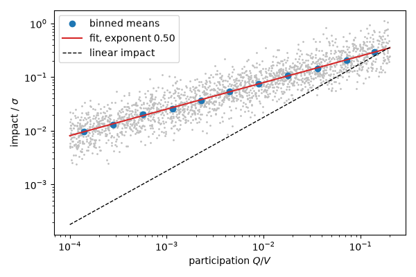
exponent 0.495 ± 0.005, Y = 0.78

Cost per share for a 2%-volatility stock

for pct in (0.1, 1, 5, 10, 25):
    print(f"{pct:5.1f}% of daily volume: {1e4 * square_root_impact(pct / 100, 1.0, 0.02):6.1f} bp")

plt.show()

 0.1% of daily volume:    6.3 bp
 1.0% of daily volume:   20.0 bp
 5.0% of daily volume:   44.7 bp
10.0% of daily volume:   63.2 bp
25.0% of daily volume:  100.0 bp