Bertsimas and Lo: optimal control of execution costs

Dimitris Bertsimas and Andrew Lo (1998) treated buying \(\bar S\) shares over \(T\) periods as a dynamic program. If each purchase moves the price permanently by \(\theta\) per share, \(P_k = P_{k-1} + \theta S_k + \varepsilon_k\), the best a risk-neutral trader can do is split the order evenly. If a serially correlated signal \(X_k\) also drives prices, the optimal order is linear in the remaining shares and the latest signal, and trading ahead of predicted rises pays.

import matplotlib.pyplot as plt
import numpy as np

from financialkit.market_microstructure import bertsimas_lo

S, T, theta = 100_000.0, 20, 5e-5
gamma, rho, sigma_eta = 0.05, 0.8, 1.0

Without information: the even split

plain = bertsimas_lo(S, T, theta)
print(f"trades {plain.trades[:3]} ..., excess cost {plain.expected_cost:.0f} = theta S^2 (T + 1) / (2T)")

trades [5000. 5000. 5000.] ..., excess cost 262500 = theta S^2 (T + 1) / (2T)

A signal tilts the schedule

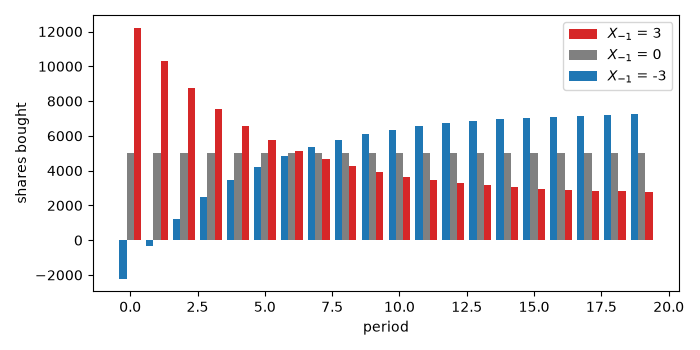
With a positive signal prices are expected to rise, so the trader buys early; with a negative one it waits.

fig, ax = plt.subplots(figsize=(7, 3.5))
k = np.arange(T)
for x0, color in [(3.0, "C3"), (0.0, "0.5"), (-3.0, "C0")]:
    ax.bar(k + 0.27 * np.sign(x0), bertsimas_lo(S, T, theta, gamma, rho, sigma_eta, x0=x0).trades, width=0.27, color=color, label=f"$X_{{-1}}$ = {x0:g}")
ax.set_xlabel("period")
ax.set_ylabel("shares bought")
ax.legend()
fig.tight_layout()

The value of reacting to the signal

Simulate the signal and prices, follow the closed-loop policy along each realised path, and compare costs with the even split.

rng = np.random.default_rng(14)
n_paths = 2000
cost_opt, cost_twap = np.empty(n_paths), np.empty(n_paths)
for j in range(n_paths):
    X = np.empty(T + 1)
    X[0] = rng.standard_normal() * sigma_eta / np.sqrt(1 - rho**2)
    for t in range(T):
        X[t + 1] = rho * X[t] + sigma_eta * rng.standard_normal()
    eps = 0.05 * rng.standard_normal(T)
    for trades, out in [(bertsimas_lo(S, T, theta, gamma, rho, sigma_eta, x0=X[0], signals=X[:-1]).trades, cost_opt), (np.full(T, S / T), cost_twap)]:
        P = np.cumsum(theta * trades + gamma * X[1:] + eps)
        out[j] = P @ trades
saving = cost_twap - cost_opt
print(f"average saving over TWAP {saving.mean():.0f} ± {saving.std() / np.sqrt(n_paths):.0f} (TWAP excess cost {plain.expected_cost:.0f})")

fig, ax = plt.subplots(figsize=(6, 3.5))
ax.hist(saving, bins=50, color="C0")
ax.axvline(0, color="k", lw=0.8)
ax.set_xlabel("cost of TWAP minus cost of the optimal policy")
fig.tight_layout()

plt.show()

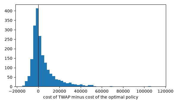
average saving over TWAP 4573 ± 289 (TWAP excess cost 262500)