Almgren and Chriss: the efficient frontier of execution

Robert Almgren and Neil Chriss (2000) split impact into a permanent part \(\gamma\) and a temporary part \(\eta\) that punishes trading fast. Selling slowly is cheap in expectation but leaves the position exposed to volatility for longer. Minimising \(E + \lambda V\) gives

\[x(t) = X \frac{\sinh(\kappa(T - t))}{\sinh(\kappa T)}, \qquad \kappa \approx \sqrt{\lambda\sigma^2/\eta},\]

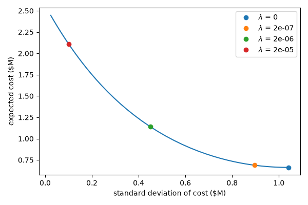
and sweeping the risk aversion \(\lambda\) traces an efficient frontier of expected cost against variance. The parameters are those of their worked example: one million shares at $50, 30% annual volatility, sold over five days.

import matplotlib.pyplot as plt
import numpy as np

from financialkit.market_microstructure import almgren_chriss
from financialkit.market_microstructure.visualizers import plot_execution

X, T, N = 1e6, 5.0, 5
sigma, eta, gamma, eps = 0.95, 2.5e-6, 2.5e-7, 0.0625

Trajectories

lams = [0.0, 2e-7, 2e-6, 2e-5]
results = [almgren_chriss(X, T, N, sigma, eta, lam, gamma, eps) for lam in lams]
ax = plot_execution(results, labels=[f"$\\lambda$ = {lam:g}" for lam in lams])
ax.set_xlabel("days")
for lam, r in zip(lams, results, strict=True):
    print(f"lambda {lam:7.0e}: E = ${r.expected_cost / 1e6:.3f}M, sd = ${np.sqrt(r.variance) / 1e6:.3f}M")

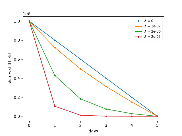
lambda   0e+00: E = $0.662M, sd = $1.041M
lambda   2e-07: E = $0.688M, sd = $0.896M
lambda   2e-06: E = $1.141M, sd = $0.449M
lambda   2e-05: E = $2.110M, sd = $0.101M

The efficient frontier

frontier = [almgren_chriss(X, T, N, sigma, eta, lam, gamma, eps) for lam in np.logspace(-8, -4, 60)]
fig, ax = plt.subplots(figsize=(6, 4))
ax.plot([np.sqrt(r.variance) / 1e6 for r in frontier], [r.expected_cost / 1e6 for r in frontier], "C0-")
for lam, r in zip(lams, results, strict=True):
    ax.plot(np.sqrt(r.variance) / 1e6, r.expected_cost / 1e6, "o", label=f"$\\lambda$ = {lam:g}")
ax.set_xlabel("standard deviation of cost ($M)")
ax.set_ylabel("expected cost ($M)")
ax.legend()
fig.tight_layout()

plt.show()