Rannacher smoothing

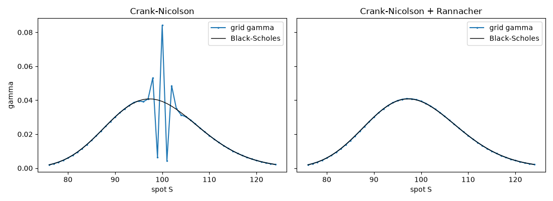
Crank-Nicolson is stable, but its amplification factor tends to \(-1\) for the stiffest modes, so the high-frequency error excited by a payoff kink is never damped: it just flips sign every step. With large time steps the price looks fine while delta and gamma oscillate around the strike. Rolf Rannacher (1984) proposed starting with a few fully implicit steps, which damp those modes, before switching to Crank-Nicolson. CrankNicolson with rannacher_steps=2 replaces the first two steps by four implicit half steps.

import matplotlib.pyplot as plt
import numpy as np

from financialkit.options import black_scholes_greeks
from financialkit.pde_methods import CrankNicolson

S, K, T, r, sigma = 100.0, 100.0, 0.25, 0.05, 0.2
plain = CrankNicolson(400, 10, s_max=400.0).price(S, K, T, r, sigma)
smooth = CrankNicolson(400, 10, rannacher_steps=2, s_max=400.0).price(S, K, T, r, sigma)
print(f"prices: plain CN {plain.price:.4f}, Rannacher {smooth.price:.4f}")

prices: plain CN 4.5980, Rannacher 4.6062

Gamma on the grid, from second differences

h = plain.S[1] - plain.S[0]
s = plain.S[1:-1]
near = (s > 75) & (s < 125)
exact = black_scholes_greeks(s[near], K, T, r, sigma).gamma
fig, axes = plt.subplots(1, 2, figsize=(11, 4), sharey=True)
for ax, res, title in ((axes[0], plain, "Crank-Nicolson"), (axes[1], smooth, "Crank-Nicolson + Rannacher")):
    ax.plot(s[near], np.diff(res.V, 2)[near] / h**2, ".-", ms=3, label="grid gamma")
    ax.plot(s[near], exact, "k", lw=1, label="Black-Scholes")
    ax.set_title(title)
    ax.set_xlabel("spot S")
    ax.legend()
axes[0].set_ylabel("gamma")
fig.tight_layout()
plt.show()