Basel historical VaR and the traffic light

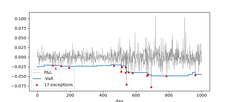
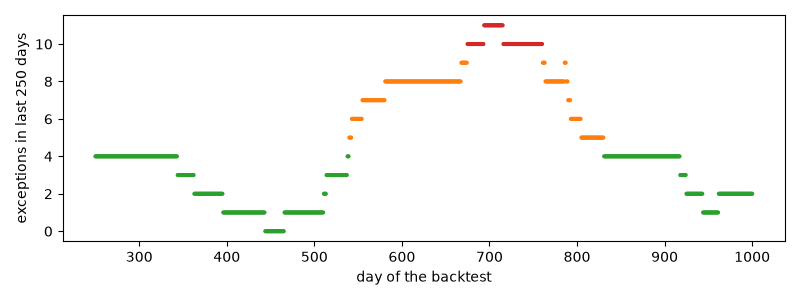
The 1996 Market Risk Amendment let banks set capital from their own 99%, ten-day VaR, typically historical simulation over at least a year of data, multiplied by at least 3. The multiplier grows with the number of exceptions in the last 250 days: green (0-4) keeps 3, yellow (5-9) adds 0.40 to 0.85, red (10 or more) adds 1. Here a historical VaR is run on a market whose volatility doubles halfway through.

import matplotlib.pyplot as plt
import numpy as np

from financialkit.risk import basel_traffic_light, rolling_historical_var, var_exceptions
from financialkit.risk.visualizers import plot_backtest

The zones

for k in range(12):
    res = basel_traffic_light(k)
    print(f"{k:2d} exceptions: {res.zone:6s} P(X <= k) = {res.cumulative_probability:.4f}  multiplier {res.multiplier:.2f}")

 0 exceptions: green  P(X <= k) = 0.0811  multiplier 3.00
 1 exceptions: green  P(X <= k) = 0.2858  multiplier 3.00
 2 exceptions: green  P(X <= k) = 0.5432  multiplier 3.00
 3 exceptions: green  P(X <= k) = 0.7581  multiplier 3.00
 4 exceptions: green  P(X <= k) = 0.8922  multiplier 3.00
 5 exceptions: yellow P(X <= k) = 0.9588  multiplier 3.40
 6 exceptions: yellow P(X <= k) = 0.9863  multiplier 3.50
 7 exceptions: yellow P(X <= k) = 0.9960  multiplier 3.65
 8 exceptions: yellow P(X <= k) = 0.9989  multiplier 3.75
 9 exceptions: yellow P(X <= k) = 0.9997  multiplier 3.85
10 exceptions: red    P(X <= k) = 0.9999  multiplier 4.00
11 exceptions: red    P(X <= k) = 1.0000  multiplier 4.00

A one-year window behind a volatility jump

rng = np.random.default_rng(7)
vol = np.r_[np.full(750, 0.01), np.full(500, 0.02)]
pnl = vol * rng.standard_t(5, vol.size) / np.sqrt(5 / 3)
window = 250
var = rolling_historical_var(pnl, window, 0.99)
test = pnl[window:]
hits = var_exceptions(test, var)
plot_backtest(test, var)

counts = np.array([hits[t - 250 : t].sum() for t in range(250, hits.size + 1)])
zones = [basel_traffic_light(int(c)).zone for c in counts]
fig, ax = plt.subplots(figsize=(8, 3))
colors = {"green": "C2", "yellow": "C1", "red": "C3"}
ax.scatter(np.arange(counts.size) + 250, counts, c=[colors[z] for z in zones], s=4)
ax.set_xlabel("day of the backtest")
ax.set_ylabel("exceptions in last 250 days")
fig.tight_layout()

plt.show()

• 
•