Artzner-Delbaen-Eber-Heath: coherent risk measures

Artzner, Delbaen, Eber and Heath (1999) listed four properties a capital requirement should have: monotonicity, subadditivity, positive homogeneity and translation invariance. VaR fails subadditivity: two desks can each look safe while their merger needs capital. The classic counterexample is a pair of independent bonds that each default with 4% probability. At 95% neither default is in the tail, so each bond’s VaR is negative; together, a default happens with probability 7.8%, and the portfolio’s VaR is a loss.

import matplotlib.pyplot as plt
import numpy as np

from financialkit.risk import ExpectedShortfall, ValueAtRisk, check_coherence

Two defaultable bonds

Each bond pays 2 if it survives and loses 100 on default. The 10,000 equally likely states reproduce the joint default probabilities exactly.

p = 0.04
n = 10_000
counts = np.round(np.array([(1 - p) ** 2, p * (1 - p), p * (1 - p), p**2]) * n).astype(int)
A = np.repeat([2.0, -100.0, 2.0, -100.0], counts)
B = np.repeat([2.0, 2.0, -100.0, -100.0], counts)

for measure in (ValueAtRisk(0.95), ExpectedShortfall(0.95)):
    res = check_coherence(measure, A, B)
    print(f"{measure.name}: rho(A) = {res.rho_x:7.2f}, rho(B) = {res.rho_y:7.2f}, rho(A + B) = {res.rho_sum:7.2f}")
    print(
        f"    subadditive {res.subadditivity}, monotone {res.monotonicity}, homogeneous {res.positive_homogeneity}, "
        f"translation invariant {res.translation_invariance}: coherent = {res.coherent}"
    )

VaR: rho(A) =   -2.00, rho(B) =   -2.00, rho(A + B) =   98.00
    subadditive False, monotone True, homogeneous True, translation invariant True: coherent = False
ES: rho(A) =   79.60, rho(B) =   79.60, rho(A + B) =  101.26
    subadditive True, monotone True, homogeneous True, translation invariant True: coherent = True

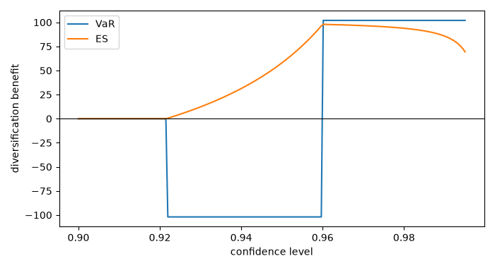
Merging gets punished, at some levels only

The diversification benefit, \(\rho(A) + \rho(B) - \rho(A + B)\), is negative for VaR at confidence levels between 92.2% and 96%, and never for ES.

levels = np.linspace(0.90, 0.995, 200)
benefit = {
    m: [(lambda r: r.rho_x + r.rho_y - r.rho_sum)(check_coherence(cls(a), A, B)) for a in levels]
    for m, cls in [("VaR", ValueAtRisk), ("ES", ExpectedShortfall)]
}
fig, ax = plt.subplots(figsize=(7, 3.8))
for m, b in benefit.items():
    ax.plot(levels, b, label=m)
ax.axhline(0, color="k", lw=0.8)
ax.set_xlabel("confidence level")
ax.set_ylabel("diversification benefit")
ax.legend()
fig.tight_layout()

plt.show()